The effects of time series length
Robert W Schlegel
2019-11-06
Last updated: 2019-11-06
workflowr checks: (Click a bullet for more information)-
✔ R Markdown file: up-to-date
Great! Since the R Markdown file has been committed to the Git repository, you know the exact version of the code that produced these results.
-
✔ Environment: empty
Great job! The global environment was empty. Objects defined in the global environment can affect the analysis in your R Markdown file in unknown ways. For reproduciblity it’s best to always run the code in an empty environment.
-
✔ Seed:
set.seed(666)The command
set.seed(666)was run prior to running the code in the R Markdown file. Setting a seed ensures that any results that rely on randomness, e.g. subsampling or permutations, are reproducible. -
✔ Session information: recorded
Great job! Recording the operating system, R version, and package versions is critical for reproducibility.
-
Great! You are using Git for version control. Tracking code development and connecting the code version to the results is critical for reproducibility. The version displayed above was the version of the Git repository at the time these results were generated.✔ Repository version: ff0bb95
Note that you need to be careful to ensure that all relevant files for the analysis have been committed to Git prior to generating the results (you can usewflow_publishorwflow_git_commit). workflowr only checks the R Markdown file, but you know if there are other scripts or data files that it depends on. Below is the status of the Git repository when the results were generated:
Note that any generated files, e.g. HTML, png, CSS, etc., are not included in this status report because it is ok for generated content to have uncommitted changes.Ignored files: Ignored: .Rhistory Ignored: .Rproj.user/ Ignored: data/global/ Ignored: data/global_results.Rda Ignored: data/global_test_trend.Rda Ignored: data/global_var_trend.Rda Ignored: data/global_var_trend_old.Rda Ignored: data/random_bp_results_100.Rda Ignored: data/random_bp_results_1000.Rda Ignored: data/random_results_100.Rda Ignored: data/random_results_1000.Rda Ignored: data/sst_ALL_bp_results.Rda Untracked files: Untracked: analysis/WA_pixels.Rda Untracked: analysis/WA_pixels_res.Rda Unstaged changes: Modified: .DS_Store Modified: .Rprofile Modified: .gitignore Modified: CODE_OF_CONDUCT.md Modified: LICENSE Modified: LICENSE.md Modified: LaTeX/FMars.csl Modified: LaTeX/Frontiers_Template.docx Modified: LaTeX/MHWdetection.docx Modified: LaTeX/MHWdetection.tex Modified: LaTeX/PDF examples/frontiers.pdf Modified: LaTeX/PDF examples/frontiers_SupplementaryMaterial.pdf Modified: LaTeX/README Modified: LaTeX/Supplementary_Material.docx Modified: LaTeX/YM-logo.eps Modified: LaTeX/fig_1.jpg Modified: LaTeX/fig_1.pdf Modified: LaTeX/fig_1_flat.jpg Modified: LaTeX/fig_1_flat.pdf Modified: LaTeX/fig_2.jpg Modified: LaTeX/fig_2.pdf Modified: LaTeX/fig_3.jpg Modified: LaTeX/fig_3.pdf Modified: LaTeX/fig_4.jpg Modified: LaTeX/fig_4.pdf Modified: LaTeX/fig_5.jpg Modified: LaTeX/fig_5.pdf Modified: LaTeX/fig_6.jpg Modified: LaTeX/fig_6.pdf Modified: LaTeX/fig_S1.jpg Modified: LaTeX/fig_S1.pdf Modified: LaTeX/fig_S2.jpg Modified: LaTeX/fig_S2.pdf Modified: LaTeX/fig_S3.jpg Modified: LaTeX/fig_S3.pdf Modified: LaTeX/fig_S4.jpg Modified: LaTeX/fig_S4.pdf Modified: LaTeX/fig_S5.jpg Modified: LaTeX/fig_S5.pdf Modified: LaTeX/figures.zip Modified: LaTeX/frontiers.tex Modified: LaTeX/frontiersFPHY.cls Modified: LaTeX/frontiersHLTH.cls Modified: LaTeX/frontiersSCNS.cls Modified: LaTeX/frontiersSCNS.log Modified: LaTeX/frontiers_SupplementaryMaterial.tex Modified: LaTeX/frontiers_suppmat.cls Modified: LaTeX/frontiersinHLTH&FPHY.bst Modified: LaTeX/frontiersinSCNS_ENG_HUMS.bst Modified: LaTeX/logo1.eps Modified: LaTeX/logo1.jpg Modified: LaTeX/logo2.eps Modified: LaTeX/logos.eps Modified: LaTeX/logos.jpg Modified: LaTeX/stfloats.sty Modified: LaTeX/table_1.xlsx Modified: LaTeX/table_2.xlsx Modified: LaTeX/test.bib Modified: MHWdetection.Rproj Modified: TODO Modified: _references/1-s2.0-S0921818106002736-main.pdf Modified: _references/1-s2.0-S092181810600275X-main.pdf Modified: _references/1-s2.0-S0921818106002761-main.pdf Modified: _references/1-s2.0-S0921818106002852-main.pdf Modified: _references/1405.3904.pdf Modified: _references/1520-0450%282001%29040%3C0762%3Aotdoah%3E2.0.co%3B2.pdf Modified: _references/2013_Extremes_Workshop_Report.pdf Modified: _references/24868781.pdf Modified: _references/24870362.pdf Modified: _references/26192647.pdf Modified: _references/994.full.pdf Modified: _references/A_1019841717369.pdf Modified: _references/Banzon et al 2014.pdf Modified: _references/Brown_et_al-2008-Journal_of_Geophysical_Research%3A_Atmospheres_%281984-2012%29.pdf Modified: _references/Different_ways_to_compute_temperature_re.pdf Modified: _references/Gilleland et al 2013.pdf Modified: _references/Gilleland_2006.pdf Modified: _references/Kuglitsch_et_al-2010-Geophysical_Research_Letters.pdf Modified: _references/Modeling Waves of Extreme Temperature The Changing Tails of Four Cities.pdf Modified: _references/Normals-Guide-to-Climate-190116_en.pdf Modified: _references/Reynolds et al 2007.pdf Modified: _references/Risk_of_Extreme_Events_Under_Nonstationa.pdf Modified: _references/Russo_et_al-2014-Journal_of_Geophysical_Research%3A_Atmospheres.pdf Modified: _references/WCDMP_72_TD_1500_en__1.pdf Modified: _references/WMO 49 v1 2015.pdf Modified: _references/WMO No 1203.pdf Modified: _references/WMO-TD No 1377.pdf Modified: _references/WMO_100_en.pdf Modified: _references/bams-d-12-00066.1.pdf Modified: _references/c058p193.pdf Modified: _references/cc100.pdf Modified: _references/clivar14.pdf Modified: _references/coles1994.pdf Modified: _references/ecology.pdf Modified: _references/joc.1141.pdf Modified: _references/joc.1432.pdf Modified: _references/returnPeriod.pdf Modified: _references/s00382-014-2287-1.pdf Modified: _references/s00382-014-2345-8.pdf Modified: _references/s00382-015-2638-6.pdf Modified: _references/s10584-006-9116-4.pdf Modified: _references/s10584-007-9392-7.pdf Modified: _references/s10584-010-9944-0.pdf Modified: _references/s10584-012-0659-2.pdf Modified: _references/s10584-014-1254-5.pdf Modified: _references/s13253-013-0161-y.pdf Modified: _references/wcrpextr.pdf Modified: _workflowr.yml Modified: analysis/Climatologies_and_baselines.Rmd Modified: analysis/Short_climatologies.Rmd Modified: analysis/about.Rmd Modified: analysis/bibliography.bib Modified: analysis/gridded_products.Rmd Modified: analysis/r_vs_python_arguments.Rmd Modified: analysis/variance.Rmd Modified: code/README.md Modified: data/.gitignore Modified: data/best_table_average.Rda Modified: data/best_table_focus.Rda Modified: data/python/clim_py.csv Modified: data/python/clim_py_joinAG_1.csv Modified: data/python/clim_py_joinAG_5.csv Modified: data/python/clim_py_joinAG_no.csv Modified: data/python/clim_py_minD_3.csv Modified: data/python/clim_py_minD_7.csv Modified: data/python/clim_py_pctile_80.csv Modified: data/python/clim_py_pctile_95.csv Modified: data/python/clim_py_pctile_99.csv Modified: data/python/clim_py_random.csv Modified: data/python/clim_py_spw_11.csv Modified: data/python/clim_py_spw_51.csv Modified: data/python/clim_py_spw_no.csv Modified: data/python/clim_py_whw_3.csv Modified: data/python/clim_py_whw_7.csv Modified: data/python/mhwBlock.csv Modified: data/python/mhws_py.csv Modified: data/python/mhws_py_joinAG_1.csv Modified: data/python/mhws_py_joinAG_5.csv Modified: data/python/mhws_py_joinAG_no.csv Modified: data/python/mhws_py_minD_3.csv Modified: data/python/mhws_py_minD_7.csv Modified: data/python/mhws_py_pctile_80.csv Modified: data/python/mhws_py_pctile_95.csv Modified: data/python/mhws_py_pctile_99.csv Modified: data/python/mhws_py_random.csv Modified: data/python/mhws_py_spw_11.csv Modified: data/python/mhws_py_spw_51.csv Modified: data/python/mhws_py_spw_no.csv Modified: data/python/mhws_py_whw_3.csv Modified: data/python/mhws_py_whw_7.csv Modified: data/python/sst_WA.csv Modified: data/python/sst_WA_miss_ice.csv Modified: data/python/sst_WA_miss_random.csv Modified: data/sst_ALL_results.Rda Modified: data/table_1.csv Modified: data/table_2.csv Modified: docs/portrait.pdf Modified: output/README.md Modified: output/effect_event.pdf Modified: output/fig_2_missing_only.pdf Modified: output/stitch_plot_WA.pdf Modified: output/stitch_sub_plot_WA.pdf Modified: poster/Figures/CSIRO_logo.jpeg Modified: poster/Figures/Dal_logo.jpg Modified: poster/Figures/all_logo_long.jpg Modified: poster/Figures/all_logos.jpg Modified: poster/Figures/logo_stitching.odp Modified: poster/Figures/ofi_logo.jpg Modified: poster/Figures/uwc-logo.jpg Modified: poster/MHWdetection.bib Modified: poster/MyBib.bib Modified: poster/landscape.Rmd Modified: poster/landscape.pdf Modified: poster/portrait.Rmd Modified: poster/portrait.pdf
Expand here to see past versions:
| File | Version | Author | Date | Message |
|---|---|---|---|---|
| Rmd | ff0bb95 | robwschlegel | 2019-11-06 | Publish the sub-optimal test vignettes |
| Rmd | f841111 | robwschlegel | 2019-11-06 | Prepped time series length vignette for website re-build |
| Rmd | fda03b2 | robwschlegel | 2019-09-03 | Beginning to dig into the methodology to answer for Reviewer 2’s comments. |
| html | b936d9f | robwschlegel | 2019-05-06 | STructure change |
| Rmd | 158aa0b | robwschlegel | 2019-05-06 | Updated project interface |
| html | 158aa0b | robwschlegel | 2019-05-06 | Updated project interface |
Overview
It has been shown that the length (count of days) of a time series may be one of the most important factors in determining the usefulness of those data for any number of applications (Schlegel and Smit 2016). For the detection of MHWs it is recommended that at least 30 years of data are used in order to accurately detect the events therein (Hobday et al. 2016). This is no longer an issue for most ocean surfaces because many high quality SST products, such as NOAA OISST, are now in exceedance of the 30-year minimum. However, besides issues relating to the coarseness of these older products, there are many other reasons why one would want to detect MHWs in products with shorter records. In situ measurements along the coast are one good example of this, another being the use of the newer higher resolution SST products, a third being the use of reanalysis/model products for the detection of events in 3D. It is therefore necessary to quantify the effects that shorter time series lengths(< 30 years) have on the detection of MHWs.
# The packages used in this analysis
library(tidyverse)
library(heatwaveR)
library(lubridate)
library(ncdf4)
library(doParallel)

# The custom functions written for the analysis
source("code/functions.R")
Time series shortening
A time series derives it’s usefulness from it’s length. This is generally because the greater the number of observations (larger sample size), the more confident one can be in the statistical outputs. This is particularly true for decadal scale measurements and is why the WMO recommends a minimum of 30 years of data before drawing any conclusions about long-term trends observed in a time series. We however want to look not at decadal scale trends, but rather at how observed MHWs compare against one another when they have been detected using longer or shorter time series. In order to to quantify this effect we will use the minimum and maximum range of time series available in the NOAA OISST product, which is 37 complete years (1982 – 2018). For comparing MHWs the minimum time series length used will be ten years so that we may still have enough events detected between shortened time series to produce robust statistics.
Before we can discuss shortening techniques, we must first consider the inherent long-term trend in the time series themselves. This is usually the primary driver for much of the event detection changes over time (Oliver et al. 2018). Therefore, if we truly want to understand the effect that a shortened time series may have on MHW detection, apart from the effect of the long-term trend, we must de-trend the time series first. To this end there is an entire separate vignette that quantifies the effect of long-term trends on the detection of events.
The WMO recommends that the period used to create a climatology be 30 years in length, starting on the first year of a decade (e.g. 1981), however; because we are going to be running these analyses on many time series shorter than 30 years, for the sake of consistency we will use all of the years present in each re-sampled time series as the climatology period, regardless of length. For example, if a time series spans 1982 – 2018, that will be the period used for calculating the climatologies. Likewise, should the time series only span the years 2006 – 2018, that will be the period used.
# The function used to de-trend the time series:
detrend <- function(df){
  resids <- broom::augment(lm(temp ~ t, df))
  res <- df %>%
    mutate(temp = round((temp - resids$.fitted),2))
  return(res)
}
The effect this has on the climatologies and MHW metrics will be quantified through the following statistics:
- The effect size of shortening will be compared against the control (30 year time series) values
- Confidence (CIs) for each MHW metric at different time series lengths will be calculated
In addition to checking all of the statistics mentioned above, it is also necessary to record what the overall relationship is with the reduction of time series length and the resultant metrics. For example, are MHWs on average more intense in shorter time series or less? This will form part of the best practice advice later.
We systematically shorten the three pre-packaged time series available in the heatwaveR package and the python distribution from 37 – 10 years on the first de-trended data. This is also run on 1000 randomly selected pixels from the global dataset, which may be seen in the script found in the GitHub repository at ‘code/workflow.R’. The full global product is also analysed but not included in the level of detail here that this sub-sample is analysed with. Only the analysis on the three reference time series is shown here due to the speed of the analysis/compiling process.
# The function used to shorten a time series
control_length <- function(year_begin, df){
  res <- df %>%
    filter(year(t) >= year_begin) %>%
    mutate(index_vals = 2018-year_begin+1,
           test = "length") %>%
    dplyr::select(test, index_vals, t, temp)
  return(res)
}
Analysis
The full analysis on the results, including the functions shown above, is run for all of the tests (time series length, missing data, and long-term trend) all at once to ensure consistency of methodology across tests. For this reason the exact step-by-step process for the time series length analysis is not laid out below. To investigate the source code one may go to ‘code/workflow.R’ in the GitHub repository. A link to that site may be found in the top right of the navigation bar for this site (the GitHub icon).
sst_ALL <- rbind(mutate(sst_WA, site = "WA"),
                 mutate(sst_NW_Atl, site = "NW_Atl"),
                 mutate(sst_Med, site = "Med"))
system.time(
  sst_ALL_results <- plyr::ddply(sst_ALL, c("site"), single_analysis, .parallel = T,
                                 full_seq = T, clim_metric = F, count_miss = T, windows = T)
) # 65 seconds
Results
A more thorough explanation of the results may be found in the manuscript. Below we show what the simple results calculated above for the effect of time series length on the duration of the average MHWs look like.
sst_ALL_results %>%
  filter(test == "length",
         var == "duration",
         id == "mean_perc") %>%
  ggplot(aes(x = index_vals, y = val, colour = site)) +
  geom_line() +
  labs(x = "Time Series Length (years)", y = "Change from control (% sum of days)", colour = "Site")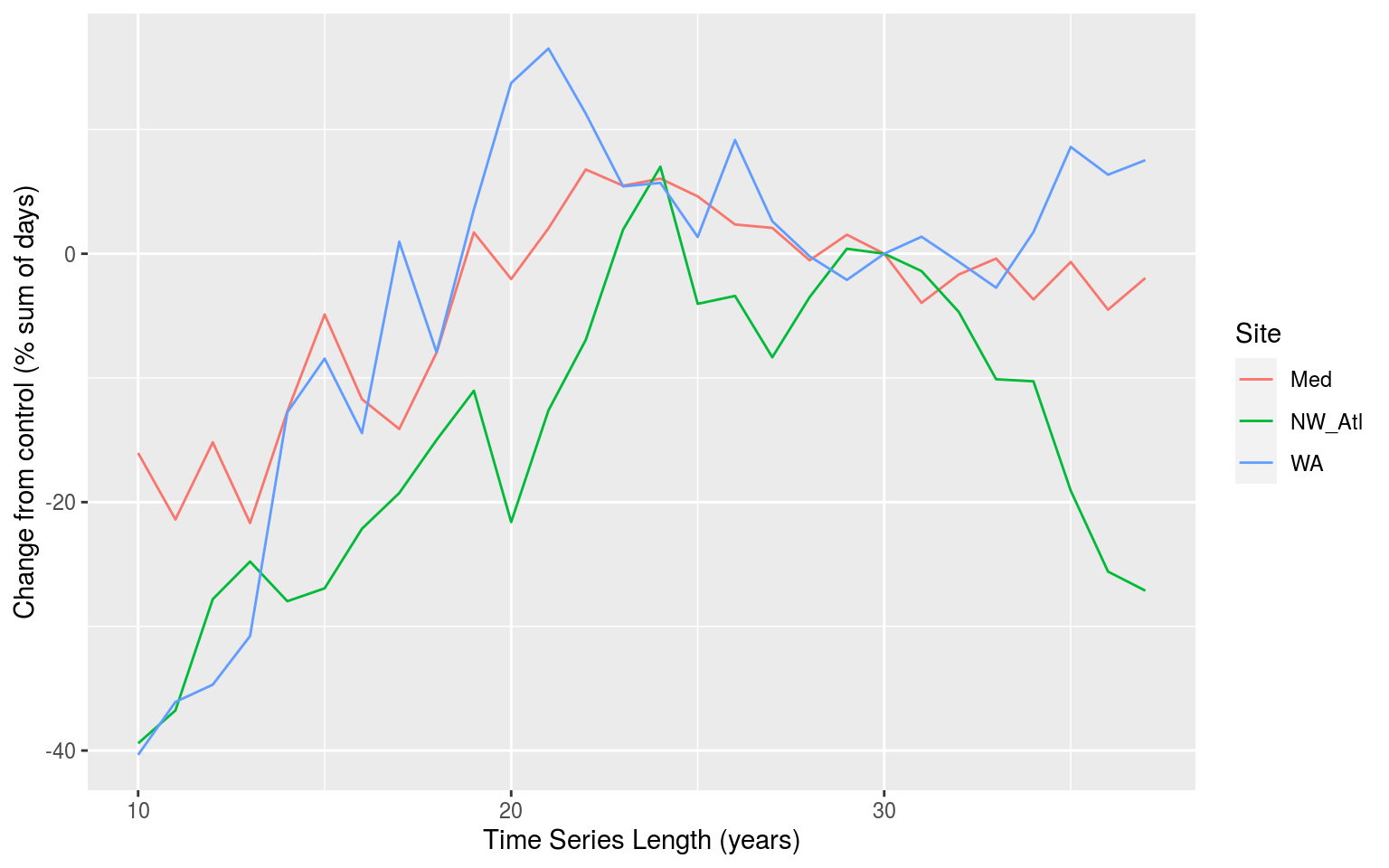
References
Hobday, Alistair J., Lisa V. Alexander, Sarah E. Perkins, Dan A. Smale, Sandra C. Straub, Eric C.J. Oliver, Jessica A. Benthuysen, et al. 2016. “A hierarchical approach to defining marine heatwaves.” Progress in Oceanography 141: 227–38. https://doi.org/10.1016/j.pocean.2015.12.014.
Oliver, Eric C.J., Markus G. Donat, Michael T. Burrows, Pippa J. Moore, Dan A. Smale, Lisa V. Alexander, Jessica A. Benthuysen, et al. 2018. “Longer and more frequent marine heatwaves over the past century.” Nature Communications 9 (1). https://doi.org/10.1038/s41467-018-03732-9.
Schlegel, Robert W., and Albertus J. Smit. 2016. “Climate Change in Coastal Waters: Time Series Properties Affecting Trend Estimation.” Journal of Climate 29 (24): 9113–24. https://doi.org/10.1175/JCLI-D-16-0014.1.
Session information
sessionInfo()R version 3.6.1 (2019-07-05)
Platform: x86_64-pc-linux-gnu (64-bit)
Running under: Ubuntu 16.04.6 LTS
Matrix products: default
BLAS: /usr/lib/openblas-base/libblas.so.3
LAPACK: /usr/lib/libopenblasp-r0.2.18.so
locale:
[1] LC_CTYPE=en_CA.UTF-8 LC_NUMERIC=C
[3] LC_TIME=en_CA.UTF-8 LC_COLLATE=en_CA.UTF-8
[5] LC_MONETARY=en_CA.UTF-8 LC_MESSAGES=en_CA.UTF-8
[7] LC_PAPER=en_CA.UTF-8 LC_NAME=C
[9] LC_ADDRESS=C LC_TELEPHONE=C
[11] LC_MEASUREMENT=en_CA.UTF-8 LC_IDENTIFICATION=C
attached base packages:
[1] parallel stats graphics grDevices utils datasets methods
[8] base
other attached packages:
[1] doParallel_1.0.15 iterators_1.0.10 foreach_1.4.4
[4] ncdf4_1.17 lubridate_1.7.4 heatwaveR_0.4.1.9003
[7] forcats_0.4.0 stringr_1.4.0 dplyr_0.8.3
[10] purrr_0.3.3 readr_1.3.1 tidyr_1.0.0
[13] tibble_2.1.3 ggplot2_3.2.1.9000 tidyverse_1.2.1
loaded via a namespace (and not attached):
[1] tidyselect_0.2.5 xfun_0.10 haven_2.1.1
[4] lattice_0.20-35 colorspace_1.4-1 vctrs_0.2.0
[7] generics_0.0.2 viridisLite_0.3.0 htmltools_0.4.0
[10] yaml_2.2.0 plotly_4.9.0 rlang_0.4.1
[13] R.oo_1.22.0 pillar_1.4.2 glue_1.3.1
[16] withr_2.1.2 R.utils_2.7.0 modelr_0.1.5
[19] readxl_1.3.1 lifecycle_0.1.0 munsell_0.5.0
[22] gtable_0.3.0 workflowr_1.1.1 cellranger_1.1.0
[25] rvest_0.3.4 R.methodsS3_1.7.1 htmlwidgets_1.5.1
[28] codetools_0.2-15 evaluate_0.14 labeling_0.3
[31] knitr_1.25 broom_0.5.2 Rcpp_1.0.2
[34] backports_1.1.5 scales_1.0.0 jsonlite_1.6
[37] hms_0.5.1 digest_0.6.22 stringi_1.4.3
[40] grid_3.6.1 rprojroot_1.3-2 cli_1.1.0
[43] tools_3.6.1 maps_3.3.0 magrittr_1.5
[46] lazyeval_0.2.2 crayon_1.3.4 whisker_0.4
[49] pkgconfig_2.0.3 zeallot_0.1.0 data.table_1.12.6
[52] xml2_1.2.2 assertthat_0.2.1 rmarkdown_1.16
[55] httr_1.4.1 rstudioapi_0.10 R6_2.4.0
[58] nlme_3.1-137 git2r_0.23.0 compiler_3.6.1 This reproducible R Markdown analysis was created with workflowr 1.1.1