
Alternative Thresholds
Robert W Schlegel
2026-04-04
Source:vignettes/complex_clims.Rmd
complex_clims.RmdOverview
The heatwaveR package was designed to
include many different methods for the creation of climatologies and
thresholds for detecting extremes events (e.g. heatwaves and
cold-spells) in time series data. To this end we made a very large
change in the event detection pipeline when we moved from the
RmarineHeatWaves package to
heatwaveR. This change may primarily be
seen with the inclusion of the ts2clm() function and the
removal of the climatology performed in
RmarineHeatWaves::detect() in favour of
detect_event(), which does not calculate climatologies. In
this way we have allowed for the introduction of a multitude of more
complex climatology calculation and event detection/filtering methods.
It is our overarching goal to provide one package that allows climate
scientists to calculate these events in both the atmosphere and oceans.
But rather than talking about it, let’s walk through some case studies
on how this package can be used for diverse applications.
Double thresholds
Brought to our attention by Mr. Haouari from the Hydrometeorological
Institute of Training and Research (IHFR) in Algeria was the concept of
using a flat
(e.g. 19C)
tMin bottom boundary when calculating events from
tMax with the standard 90th percentile upper threshold. As
the authors of the heatwaveR package are
admittedly marine oriented, we tend to work with daily time series that
have only one mean value per day (e.g. tMean,
temp, sst). This is why there are not
arguments in the heatwaveR suite of
functions that call on tMin and tMax
explicitly, but that does not mean that one cannot do so. Below we will
work through the steps one would take to calculate (atmospheric)
heatwaves, as per their definition in Perkins and
Alexander (2013) (but excluding the calculation of EHF), and with
the additional step proposed by Mr. Haouari.
The following sub-sections will show the step-by-step process one may
use to calculate atmospheric heatwaves using a 90th percentile threshold
created from the tMax time series for a location, but will
only use the days when the corresponding tMin also exceeds
a pre-determined flat bottom boundary on the same days to quantify the
heatwave metrics. We will finish by visualising the results with the
built-in heatwaveR graphing functions of
event_line() and lolli_plot as well as a
bubble plot. The data we will use for these examples will be a 45 year
time series of daily atmospheric tMin and tMax
temperatures over Algiers, Algeria contributed by Mr. Haouari.
Data prep
The first step with any analysis in R should be the loading of the packages to be used.
With our libraries loaded, we will now go about explicitly calling
the Algiers data into our environment. These data are
automatically loaded for us when we load the heatwaveR
library, but we perform this step here just for clarity. Anyone
following along should feel free to use whatever data they would like.
As long as the data have a date (t), tMin, and
tMax column this code will function as designed.
Algiers <- AlgiersCalculating thresholds
With our libraries and data loaded, we will now calculate the two
thresholds we need to correctly detect the heatwaves and accurately
quantify their metrics. The first is the 90th percentile threshold based
on the tMax time series. The second is the flat exceedance
of
19C
based on the tMin data. We use
19C
as the bottom threshold as this is roughly the mean tMin
for summer temperatures.
# The tMax threshold
# The current WMO standard climatology period is 1981-01-01 to 2010-12-31 and should be used when possible
# We rather use 1961-01-01 to 1990-01-01 as this is the oldest 30 year period available in the data
tMax_clim <- ts2clm(data = Algiers, y = tMax, climatologyPeriod = c("1961-01-01", "1990-12-31"), pctile = 90)

# The tMin exceedance
# Note the use here of 'minDuration = 3' and 'maxGap = 1' as the default atmospheric arguments
# The default marine arguments are 'minDuration = 5' and 'maxGap = 2'
tMin_exc <- exceedance(data = Algiers, y = tMin, threshold = 19, minDuration = 3, maxGap = 1)$threshold
Calculating events
Now that the two thresholds have been calculated we use the
detect_event() function as usual, but provide the second
threshold to the argument threshClim2 that would normally
lay dormant.
# Note that because we calculated our 90th percentile threshold on a column named 'tMax'
# and not the default column name 'temp', we must specify this below with 'y = tMax'
events <- detect_event(data = tMax_clim, y = tMax, # The 90th percentile threshold
                       threshClim2 = tMin_exc$exceedance) # The flat exceedance threshold
Please note that even though the use of the second threshold does
allow for the resultant event metrics to differ, the values themselves
are still being calculated against the seasonal climatology and daily
temperatures for the time series given to the 90th percentile threshold
calculation (in this case tMax) and so using a second
threshold (in this case tMin) won’t generally have much of
an effect on the event metrics. Rather it mostly screens out smaller or
larger events depending on how one chooses to set the threshold. In the
case when an exceedance threshold is chosen for a temperature that would
typically only occur in summer
(e.g. 19C,
as used here), one is also effectively screening events by season. There
are many use cases where this would be desirable. For example, if one is
only interested in events that would occur during a season in which
night time heat stress becomes an issue for the young and elderly.
Creating visuals
Even though we have used two thresholds to calculate our events, the
results are output the same as though only one threshold (default) were
used. This means that we may use the visualisation functions that come
with heatwaveR without any extra fuss.
# The code to create a bubble plot for the heatwave results
bubble_plot <- ggplot(data = events$event, aes(x = date_peak, y = intensity_max)) +
  geom_point(aes(size = intensity_cumulative), shape = 21, fill = "salmon", alpha = 0.8) +
  labs(x = NULL, y = "Maximum Intensity [°C] ", size = "Cumulative Intensity [°C x days]") +
  scale_size_continuous(range = c(1, 10),
                        guide = guide_legend(title.position = "top", direction = "horizontal")) +
  theme_bw() +
  theme(legend.position = c(0.3, 0.12),
        legend.box.background = element_rect(colour = "black"))

# Don't forget to set 'event_line(y = tMax)'
ggarrange(event_line(events, y = tMax, metric = intensity_max),
          event_line(events, y = tMax, metric = intensity_max, category = T),
          lolli_plot(events),
          bubble_plot,
          ncol = 2, nrow = 2, align = "hv")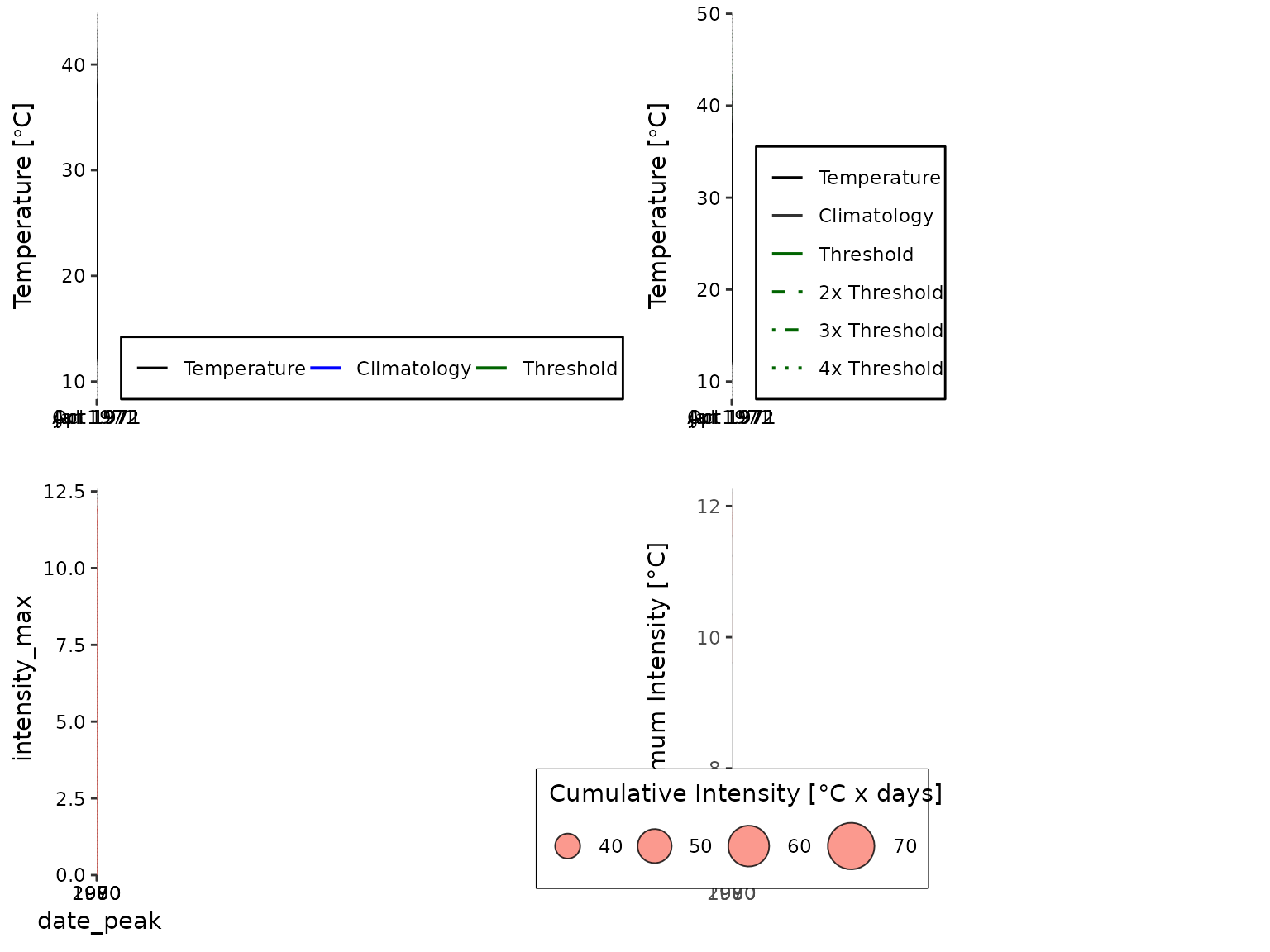
Alternative second thresholds
Using a percentile based second threshold is not much different than
using a static second threshold. Rather than using
exceedance() to get our second threshold we can use
ts2clm nested within detect_event(). It must
also be pointed out that in addition to using multiple thresholds, we
can adjust the minimum duration (minDuration) and maximum
gap (maxGap) arguments for our multiple thresholds, too.
This allows us to provide different ‘flavours’ of criteria for our
events. For example, let’s say we are interested in night-time events
(tMin) when the temperatures remain above the 80th
percentile threshold (pctile = 80) for 10 or more days
(minDuration = 10) without dipping below that threshold for
more than 2 consecutive days (maxGap = 2). But on top of
that, we are also only interested in those parts of the event when the
daytime temperatures exceed the 90th percentile threshold
(pctile = 90) for 3 or more days
(minDuration = 3) non-stop (maxGap = 0).
Below we will look at how to detect/calculate events that meet these
rather specific criteria. We will also calculate events with just the
first threshold and compare the results visually. It must be noted here
that whichever criteria is the most strict, in this case
minDuration = 3 and maxGap = 0, will be the
predominant filter through which the event metrics are quantified.
# Note that because we are not using the standard column name 'temp' we must
# specify the chosen column name twice, once for ts2clm() and again for detect_event()

# First threshold based on tMin
thresh_tMin <- ts2clm(data = Algiers, y = tMin, pctile = 80,
                      climatologyPeriod = c("1961-01-01", "1990-12-31"))

# Second threshold based on tMax
# Be careful here that you put the arguments within the correct brackets
thresh_tMax <- detect_event(ts2clm(data = Algiers, y = tMax, pctile = 90,
                                   climatologyPeriod = c("1961-01-01", "1990-12-31")),
                            # These arguments are passed to detect_event(), not ts2clm()
                            minDuration = 3, maxGap = 0, y = tMax, protoEvents = T)

# Detect/calculate events using the two precalculated thresholds
# Because detect_event() is not able to deduce which arguments we used above,
# we must again tell it explicitly here
events_two_thresh <- detect_event(data = thresh_tMin, y = tMin, minDuration = 10, maxGap = 2,
                                  threshClim2 = thresh_tMax$event, minDuration2 = 3, maxGap2 = 0)

# Or to simply use one threshold
events_one_thresh <- detect_event(data = thresh_tMin, y = tMin, minDuration = 10, maxGap = 2)
Here are the differences in lolliplot format:
ggarrange(lolli_plot(events_one_thresh), lolli_plot(events_two_thresh), labels = c("One threshold", "Two thresholds"))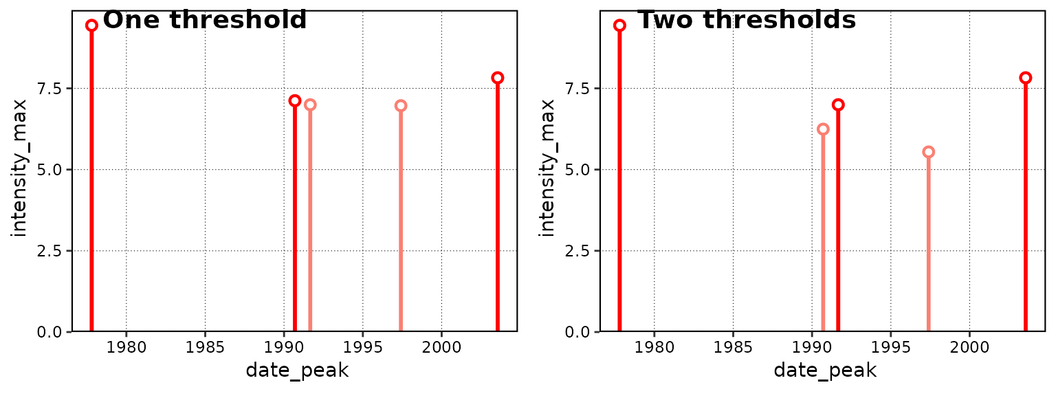
Here is a brief display of the top few events from each method:
head(events_one_thresh$event)## event_no index_start index_peak index_end duration date_start date_peak
## 1 1 6135 6137 6144 10 1977-10-18 1977-10-20
## 2 2 10844 10845 10856 13 1990-09-09 1990-09-10
## 3 3 11191 11200 11201 11 1991-08-22 1991-08-31
## 4 4 13292 13300 13301 10 1997-05-23 1997-05-31
## 5 5 15534 15542 15546 13 2003-07-13 2003-07-21
## date_end intensity_mean intensity_max intensity_var intensity_cumulative
## 1 1977-10-27 6.3138 9.4382 2.2112 63.1381
## 2 1990-09-21 4.8424 7.1201 1.1790 62.9507
## 3 1991-09-01 4.2121 6.9957 1.3819 46.3328
## 4 1997-06-01 5.1003 6.9670 1.4467 51.0026
## 5 2003-07-25 4.9539 7.8255 1.5317 64.4012
## intensity_mean_relThresh intensity_max_relThresh intensity_var_relThresh
## 1 3.7265 6.8697 2.2268
## 2 2.1077 4.3639 1.1767
## 3 1.5352 4.2877 1.3602
## 4 2.3915 4.3123 1.4514
## 5 2.4188 5.3032 1.5337
## intensity_cumulative_relThresh intensity_mean_abs intensity_max_abs
## 1 37.2652 19.1700 22.6
## 2 27.4000 21.9538 24.6
## 3 16.8871 22.6091 25.1
## 4 23.9148 18.4400 20.7
## 5 31.4441 23.6154 26.6
## intensity_var_abs intensity_cumulative_abs rate_onset rate_decline
## 1 2.4454 191.7 2.7282 0.8901
## 2 1.2474 285.4 2.9576 0.3342
## 3 1.2169 248.7 0.5665 2.5287
## 4 1.5284 184.4 0.6922 3.4156
## 5 1.5737 307.0 0.6559 1.2658
head(events_two_thresh$event)## event_no index_start index_peak index_end duration date_start date_peak
## 1 1 6135 6137 6137 3 1977-10-18 1977-10-20
## 2 2 10851 10851 10856 6 1990-09-16 1990-09-16
## 3 3 11191 11200 11201 11 1991-08-22 1991-08-31
## 4 4 13292 13294 13294 3 1997-05-23 1997-05-25
## 5 5 15540 15542 15545 6 2003-07-19 2003-07-21
## date_end intensity_mean intensity_max intensity_var intensity_cumulative
## 1 1977-10-20 7.8121 9.4382 1.6787 23.4362
## 2 1990-09-21 4.6254 6.2445 1.1706 27.7521
## 3 1991-09-01 4.2121 6.9957 1.3819 46.3328
## 4 1997-05-25 4.5271 5.5434 1.0897 13.5814
## 5 2003-07-24 5.5217 7.8255 1.6801 33.1301
## intensity_mean_relThresh intensity_max_relThresh intensity_var_relThresh
## 1 5.2521 6.8697 1.6710
## 2 1.9070 3.5148 1.1701
## 3 1.5352 4.2877 1.3602
## 4 1.7688 2.7948 1.0998
## 5 3.0012 5.3032 1.6827
## intensity_cumulative_relThresh intensity_mean_abs intensity_max_abs
## 1 15.7562 21.1000 22.6
## 2 11.4419 21.4667 23.3
## 3 16.8871 22.6091 25.1
## 4 5.3064 17.4667 18.6
## 5 18.0071 24.3167 26.6
## intensity_var_abs intensity_cumulative_abs rate_onset rate_decline
## 1 1.5524 63.3 2.7282 1.9769
## 2 1.1776 128.8 0.9760 0.5396
## 3 1.2169 248.7 0.5665 2.5287
## 4 1.2055 52.4 1.7839 0.1172
## 5 1.7034 145.9 0.7293 1.0585If we look at these results we see that the use of two thresholds did not detected fewer events than the use of one threshold. This is because even though the second threshold was much more ‘difficult’ for the time series to surpass than the first, the heatwaves in the time series are so pronounced that they emerge regardless. This method allows for a lot of flexibility, but users should also be cautious that they understand what exactly they are asking their machines to do. In the case above, it may be that we would actually prefer to calculate our event metrics based entirely on the first threshold, but filter out the events that didn’t meet our second threshold criteria. We will see how to do this in the following section.
Filtering with a second threshold
The methodology outlined below for the detection and filtering of
events with two thresholds is somewhat cumbersome. A potential issue
with this technique is that the multiple filters do not affect the
calculation of the event metrics
(e.g. intensity_cumulative), as only the primary threshold
given to detect_event() is used when calculating event
metrics. This may however be the desired case if one is still interested
in knowing the cumulative intensity above the given percentile
threshold, but only wants to filter the full event based on some other
threshold criteria. I can imagine real-world use cases for both
scenarios, which is why this seemingly less sophisticated approach is
detailed below.
Filtering events
Because we have already calculated our single threshold events
(events_one_thresh) and our second threshold
(thresh_tMax) we may directly begin filtering the results.
Before we do so, let’s pull out the list components of our results into
dataframes for easier use down the line.
# Pull out each data.frame as their own object for easier use
events_one_event <- events_one_thresh$event
events_one_climatology <- events_one_thresh$climatology
This is where things may get tricky for some users, and where the
default use of the functions in the
heatwaveR package ends. We are now going
‘off-road’ so to speak. But do not despair! The
tidyverse suite of packages makes data
wrangling like this much more user friendly than it was in the dark days
of Base R coding.
In order to make the filtering of events easier, we will combine the two different dataframes that we are using as threshold/filtering guides to chose the events that meet all of our selection criteria.
# Join the two threshold dataframes
two_thresh <- left_join(events_one_climatology, thresh_tMax, by = c("t"))

# Remove all days that did not qualify as events in both thresholds
two_thresh_filtered <- two_thresh %>%
  filter(event.x == TRUE,
         event.y == TRUE)
With our filtering guide created, we may now apply it to
events_one_thresh to get our filtered results.
# Copy data with a new name
events_one_thresh_filtered <- events_one_thresh

# Then filter
events_one_thresh_filtered$event <- events_one_thresh_filtered$event %>%
  filter(event_no %in% two_thresh_filtered$event_no.x)

# Compare results
head(events_one_thresh_filtered$event)
## event_no index_start index_peak index_end duration date_start date_peak
## 1 1 6135 6137 6144 10 1977-10-18 1977-10-20
## 2 2 10844 10845 10856 13 1990-09-09 1990-09-10
## 3 3 11191 11200 11201 11 1991-08-22 1991-08-31
## 4 4 13292 13300 13301 10 1997-05-23 1997-05-31
## 5 5 15534 15542 15546 13 2003-07-13 2003-07-21
## date_end intensity_mean intensity_max intensity_var intensity_cumulative
## 1 1977-10-27 6.3138 9.4382 2.2112 63.1381
## 2 1990-09-21 4.8424 7.1201 1.1790 62.9507
## 3 1991-09-01 4.2121 6.9957 1.3819 46.3328
## 4 1997-06-01 5.1003 6.9670 1.4467 51.0026
## 5 2003-07-25 4.9539 7.8255 1.5317 64.4012
## intensity_mean_relThresh intensity_max_relThresh intensity_var_relThresh
## 1 3.7265 6.8697 2.2268
## 2 2.1077 4.3639 1.1767
## 3 1.5352 4.2877 1.3602
## 4 2.3915 4.3123 1.4514
## 5 2.4188 5.3032 1.5337
## intensity_cumulative_relThresh intensity_mean_abs intensity_max_abs
## 1 37.2652 19.1700 22.6
## 2 27.4000 21.9538 24.6
## 3 16.8871 22.6091 25.1
## 4 23.9148 18.4400 20.7
## 5 31.4441 23.6154 26.6
## intensity_var_abs intensity_cumulative_abs rate_onset rate_decline
## 1 2.4454 191.7 2.7282 0.8901
## 2 1.2474 285.4 2.9576 0.3342
## 3 1.2169 248.7 0.5665 2.5287
## 4 1.5284 184.4 0.6922 3.4156
## 5 1.5737 307.0 0.6559 1.2658
head(events_two_thresh$event)## event_no index_start index_peak index_end duration date_start date_peak
## 1 1 6135 6137 6137 3 1977-10-18 1977-10-20
## 2 2 10851 10851 10856 6 1990-09-16 1990-09-16
## 3 3 11191 11200 11201 11 1991-08-22 1991-08-31
## 4 4 13292 13294 13294 3 1997-05-23 1997-05-25
## 5 5 15540 15542 15545 6 2003-07-19 2003-07-21
## date_end intensity_mean intensity_max intensity_var intensity_cumulative
## 1 1977-10-20 7.8121 9.4382 1.6787 23.4362
## 2 1990-09-21 4.6254 6.2445 1.1706 27.7521
## 3 1991-09-01 4.2121 6.9957 1.3819 46.3328
## 4 1997-05-25 4.5271 5.5434 1.0897 13.5814
## 5 2003-07-24 5.5217 7.8255 1.6801 33.1301
## intensity_mean_relThresh intensity_max_relThresh intensity_var_relThresh
## 1 5.2521 6.8697 1.6710
## 2 1.9070 3.5148 1.1701
## 3 1.5352 4.2877 1.3602
## 4 1.7688 2.7948 1.0998
## 5 3.0012 5.3032 1.6827
## intensity_cumulative_relThresh intensity_mean_abs intensity_max_abs
## 1 15.7562 21.1000 22.6
## 2 11.4419 21.4667 23.3
## 3 16.8871 22.6091 25.1
## 4 5.3064 17.4667 18.6
## 5 18.0071 24.3167 26.6
## intensity_var_abs intensity_cumulative_abs rate_onset rate_decline
## 1 1.5524 63.3 2.7282 1.9769
## 2 1.1776 128.8 0.9760 0.5396
## 3 1.2169 248.7 0.5665 2.5287
## 4 1.2055 52.4 1.7839 0.1172
## 5 1.7034 145.9 0.7293 1.0585The event numbers found in events_one_thresh_filtered
are the same as the event numbers found in
events_two_thresh with the important difference that the
event metrics in events_two_thresh were calculated only on
the days that exceeded both thresholds, while the events in
events_one_thresh_filtered have had their metrics
calculated from all of the days that exceeded only the first
threshold.
Visualising filtered events
To better understand how different the results from these two different techniques may be we will use lolliplots to visualise them.
ggarrange(lolli_plot(events_two_thresh, metric = duration),
          lolli_plot(events_one_thresh_filtered, metric = duration),
          labels = c("Double threshold", "Filter threshold"))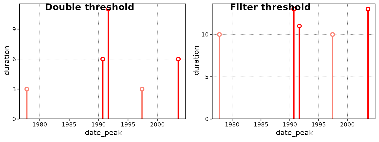
Difference in duration (days) of events given different applications of thresholds. Note the difference in the y-axes.
ggarrange(lolli_plot(events_two_thresh, metric = intensity_cumulative),
          lolli_plot(events_one_thresh_filtered, metric = intensity_cumulative),
          labels = c("Double threshold", "Filter threshold"))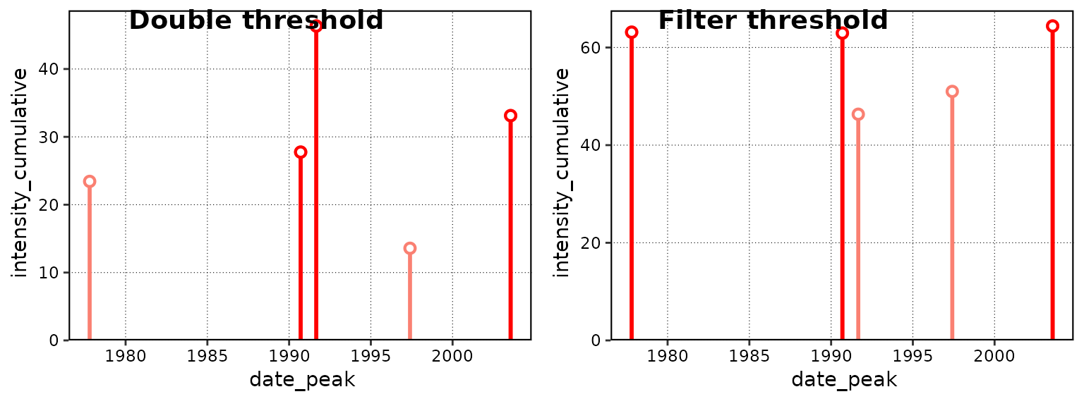
Difference in cumulative intensity (°C x days) of events given different applications of thresholds. Note the difference in the y-axes.
One may of course visualise the outputs from the events calculated
here with geom_flame() and geom_lolli() as
well, but this will not differ from the default method of using these
functions as outlined in their help files so we will not go into that
here.
Summary
This vignette serves as a guideline for how to implement multiple
methodologies for using two thresholds (tMin and
tMax) with atmospheric data. We also showed in this
vignette a more straight forward approach to using a second threshold
through the built-in arguments in detect_event(). The use
of a second threshold in this way, whether it be based on a static
threshold or one derived from a percentile, is useful for the
consideration of events that may be more specifically relevant to a
given season or organism.
I hope the techniques shown in this vignette will be useful both
technically and theoretically. The authors of
heatwaveR are very happy to receive any
further input on the development of the package as well as other
potential methods for calculating heatwaves and cold-spells in air or
sea.