4D blob connectivity: heatwaves through the water column • heatwave3

Overview

detect_blob3() finds spatially contiguous marine heatwave “blobs” by connected-component labelling of the daily exceedance mask. Given a depth-resolved climatology (from ts2clm3(depth_range = ...), see vignette("depth-range")), it now does this natively in 4D: a voxel connects to its neighbours in longitude, latitude, depth, and time, instead of just the first three. No new argument is needed – exactly like detect_event3() and category_daily3(), detect_blob3() reads the depth range straight off clim_file and switches to 4D connectivity automatically.

Connectivity is by depth index, not a depth range. A voxel connects to whichever level is immediately above or below it – level 3 to level 4, say – regardless of how many metres apart those levels actually are. There is no minimum/maximum vertical gap or distance threshold: two voxels one level apart always connect if both exceed the threshold that day; two voxels separated by an empty level in between never do, however close together in metres those levels happen to be. This mirrors exactly how the existing lon/lat/time connectivity already works (adjacent index, not adjacent degrees or adjacent days-within-some-window).

This vignette uses the small 2x2 pixel, 5 depth-level GLORYS fixture bundled with the package (system.file("extdata/glorys_depth_test.nc", package = "heatwave3")). The trade-off: with only 4 horizontal pixels, this fixture can’t show interesting spatial footprints. What it can show clearly is the vertical structure this section adds – a blob’s footprint growing and shrinking through the water column over its lifetime.

library(heatwave3)
library(ggplot2)

f <- system.file("extdata/glorys_depth_test.nc", package = "heatwave3")

Detecting depth-connected blobs

First, a depth-resolved climatology covering all 5 levels in the fixture (0.49-5.08 m):

stem <- file.path(tempdir(), "mhw4d")
ts2clm3(f, name = stem,
        climatologyPeriod = c("1993-01-01", "2019-12-31"),
        depth_range = c(0, 10), 
        quiet = TRUE)

Show console output

#> Reading SST data from /tmp/RtmpxYwdBf/temp_libpath94004dd393d4/heatwave3/extdata/glorys_depth_test.nc...
#> Grid: 2 lon x 2 lat x 5 depth x 11688 time = 20 pixels
#> Computing climatology with 1 thread(s)...
#>   1/20 pixels (5%)  2/20 pixels (10%)  3/20 pixels (15%)  4/20 pixels (20%)  5/20 pixels (25%)  6/20 pixels (30%)  7/20 pixels (35%)  8/20 pixels (40%)  9/20 pixels (45%)  10/20 pixels (50%)  11/20 pixels (55%)  12/20 pixels (60%)  13/20 pixels (65%)  14/20 pixels (70%)  15/20 pixels (75%)  16/20 pixels (80%)  17/20 pixels (85%)  18/20 pixels (90%)  19/20 pixels (95%)  20/20 pixels (100%)
#> Writing climatology to /tmp/RtmpPbzxzr/mhw4d_clim.nc...
#> Done.

detect_blob3() picks up the depth dimension from stem_clim.nc automatically:

blobs <- detect_blob3(f, paste0(stem, "_clim.nc"),
                      minVoxels = 1,
                      return = c("event", "daily", "voxel"))
nrow(blobs$event)
#> [1] 412

event and daily both gain depth/volume columns; voxel gains a depth column:

names(blobs$event)
#>  [1] "blob"                   "duration"               "date_start"            
#>  [4] "date_end"               "date_peak"              "cumI_km2_day"          
#>  [7] "peakArea_km2"           "meanArea_km2"           "centroid_lon"          
#> [10] "centroid_lat"           "depth_min_m"            "depth_max_m"           
#> [13] "totalVolume_km3"        "peakVolume_km3"         "meanVolume_km3"        
#> [16] "depthOfPeakIntensity_m" "rank"
names(blobs$daily)
#>  [1] "blob"                 "t_idx"                "area_km2"            
#>  [4] "mean_delta"           "max_delta"            "centroid_lon"        
#>  [7] "centroid_lat"         "lon_min"              "lon_max"             
#> [10] "lat_min"              "lat_max"              "n_cells"             
#> [13] "volume_km3"           "depth_min_m"          "depth_max_m"         
#> [16] "depth_at_max_delta_m" "date"

depth_min_m/depth_max_m are each blob’s vertical bounding box over its whole lifetime; totalVolume_km3/peakVolume_km3/meanVolume_km3 are the volumetric analogues of the existing cumI_km2_day/peakArea_km2/ meanArea_km2 area metrics (volume = area x vertical layer thickness, summed over the depth levels a blob occupies that day); depthOfPeakIntensity_m is the depth at which the single most intense day of the blob’s life occurred. rankBy accepts the volume metrics too when the input is depth-resolved:

top <- detect_blob3(f, paste0(stem, "_clim.nc"),
                    topN = 5, rankBy = "totalVolume_km3", return = "event")
top$event[, c("blob", "rank", "duration", "depth_min_m", "depth_max_m",
             "totalVolume_km3")]
#>   blob rank duration depth_min_m depth_max_m totalVolume_km3
#> 1   54    1       28    0.494025    5.078224        39.29278
#> 2   67    2       22    0.494025    5.078224        35.64613
#> 3   85    3       24    0.494025    5.078224        34.02462
#> 4  390    4       23    0.494025    5.078224        33.61934
#> 5  291    5       24    0.494025    5.078224        33.60915

How much does depth connectivity actually change?

The direct way to see the effect: for how many blobs does the vertical bounding box span more than a single level (depth_min_m != depth_max_m)? If depth connectivity did nothing, this would always be zero – every blob would be confined to the one level it was seeded on.

spans_multiple <- blobs$event$depth_min_m != blobs$event$depth_max_m
mean(spans_multiple)
#> [1] 0.9660194
sum(spans_multiple)
#> [1] 398

On this fixture, the large majority of blobs span more than one depth level – voxels at adjacent levels are genuinely being unioned into shared blobs, not kept artificially separate per level.

Visualising a blob’s vertical extent over time

Pick one blob and look at how its depth range and volume evolve day by day, using the daily table:

b <- top$event$blob[1]
dd <- blobs$daily[blobs$daily$blob == b, ]
range(dd$date)
#> [1] "1999-05-31" "1999-06-27"

ggplot(dd, aes(x = date)) +
  geom_ribbon(aes(ymin = depth_min_m, ymax = depth_max_m, fill = mean_delta)) +
  scale_y_reverse(name = "depth (m)") +
  scale_fill_viridis_c(name = expression(Delta*"T (" * degree * "C)"), option = "inferno") +
  labs(title = paste("Vertical extent of blob", b), x = NULL) +
  theme_minimal(base_size = 11)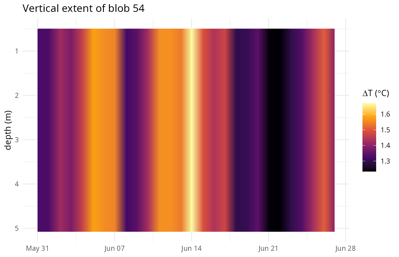

Any day where the ribbon narrows (or a depth level briefly drops out entirely) is a day the blob temporarily loses part of its vertical extent – some level’s exceedance broke the connection to the surface (or the deep levels) that day, then reconnected once conditions there crossed the threshold again. Note that in this example however there are no missing values.

Depth-time structure of a single blob

The voxel table gives the full per-voxel footprint, which – aggregated across this fixture’s 5 horizontal pixels since they’re not the interesting axis here – makes a genuine depth-time “Hovmoeller” view of one blob’s water column:

vox <- blobs$voxel[blobs$voxel$blob == b, ]
agg <- aggregate(delta ~ date + depth, data = vox, FUN = mean)

ggplot(agg, aes(x = date, y = depth, fill = delta)) +
  geom_tile() +
  scale_y_reverse(name = "depth (m)") +
  scale_fill_viridis_c(name = expression(Delta*"T (" * degree * "C)"), option = "inferno") +
  labs(title = paste("Depth-time structure of blob", b), x = NULL) +
  theme_minimal(base_size = 11)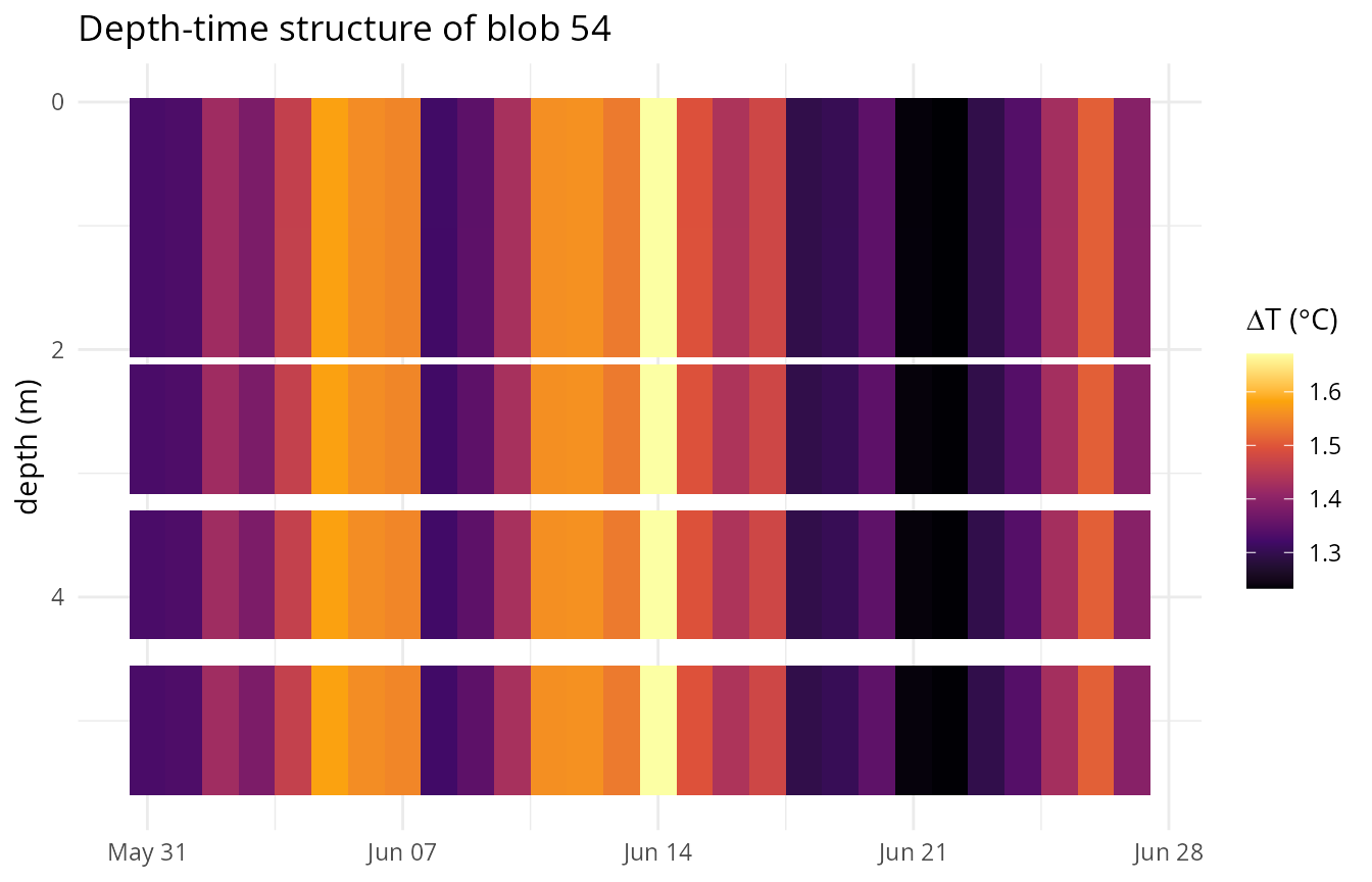

The gaps (white tiles) are days/levels that didn’t exceed the threshold that day and so aren’t part of the blob – exactly the same days visible as notches in the ribbon plot above, just resolved to the individual level rather than a min/max envelope. Note however that for this example there are no gaps, the distance between the tiles is due to the increasing size of the depth layers.