
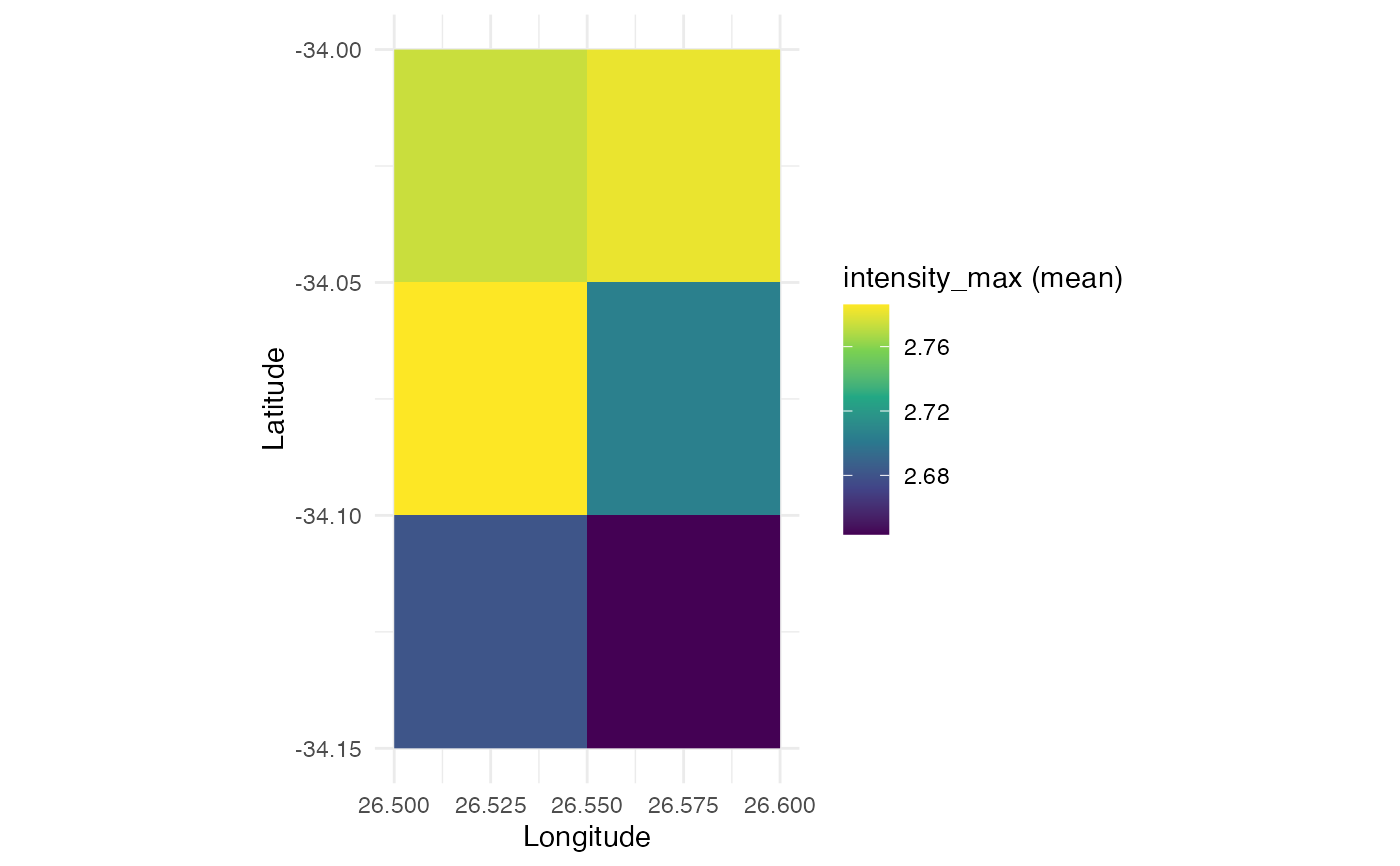
Creates a map showing the spatial distribution of a chosen event metric from the event NetCDF output. The per-pixel aggregation is performed in C++ for efficiency; the R layer handles only the ggplot2 rendering.
Arguments
- event_file
Path to the event NetCDF file from
detect_event3.- metric
Character. The event metric to map. Options include
"intensity_max"(default),"intensity_mean","intensity_cumulative","duration","rate_onset","rate_decline", and allrelThresh/absvariants.- summary
Character. How to aggregate across events per pixel. One of
"mean"(default),"max","min","sum", or"count".- coastline
Logical. Add a coastline layer? Requires the
rnaturalearth,rnaturalearthdataandsfpackages (skipped otherwise). DefaultTRUE.- ...
Additional arguments passed to
ggplot2::scale_fill_viridis_c.
Value
A ggplot object. The underlying data is accessible via
ggplot2::layer_data() or by calling
hw3_read_metric_summary() directly.
Examples
# \donttest{
sst_file <- system.file("extdata/sst_test.nc", package = "heatwave3")
stem <- file.path(tempdir(), "demo")
detect3(sst_file, name = stem,
climatologyPeriod = c("1982-01-01", "2011-12-31"))
#> Reading SST data from /Users/rschlegel/Library/R/arm64/4.6/library/heatwave3/extdata/sst_test.nc...
#> Grid: 2 lon x 3 lat x 14276 time = 6 pixels
#> Computing climatology with 1 thread(s)...
#>
1/6 pixels (16%)
2/6 pixels (33%)
3/6 pixels (50%)
4/6 pixels (66%)
5/6 pixels (83%)
6/6 pixels (100%)
#> Writing climatology to /var/folders/w8/8kw9l4sx1v57nx6l9s0rrklw0000gp/T//Rtmpe7lMQ4/demo_clim.nc...
#> Done.
#>
#> ------------------------------------------------------------------
#> Climatology written to: /var/folders/w8/8kw9l4sx1v57nx6l9s0rrklw0000gp/T//Rtmpe7lMQ4/demo_clim.nc
#> Rows (long format): 2,196 grid: 2 lon x 3 lat
#>
#> Head:
#> lon lat doy seas thresh
#> 1 26.525 -34.125 1 294.4175 295.9932
#> 2 26.525 -34.125 2 294.4615 296.0291
#> 3 26.525 -34.125 3 294.5055 296.0700
#> 4 26.525 -34.125 4 294.5491 296.1114
#> 5 26.525 -34.125 5 294.5922 296.1533
#>
#> Tail:
#> lon lat doy seas thresh
#> 2192 26.575 -34.025 362 293.5284 295.1877
#> 2193 26.575 -34.025 363 293.5648 295.2171
#> 2194 26.575 -34.025 364 293.6041 295.2490
#> 2195 26.575 -34.025 365 293.6456 295.2806
#> 2196 26.575 -34.025 366 293.6883 295.3129
#>
#> Summary:
#> ocean pixels (valid climatology): 6
#> seas: 291.1 to 295.6
#> thresh: 292.4 to 297.6
#>
#> Examine with hw3_export("/var/folders/w8/8kw9l4sx1v57nx6l9s0rrklw0000gp/T//Rtmpe7lMQ4/demo_clim.nc", n = 20)
#> or export with hw3_export("/var/folders/w8/8kw9l4sx1v57nx6l9s0rrklw0000gp/T//Rtmpe7lMQ4/demo_clim.nc", file_out = "out.csv") (.csv/.rds/.parquet)
#> ------------------------------------------------------------------
#> Reading climatology from /var/folders/w8/8kw9l4sx1v57nx6l9s0rrklw0000gp/T//Rtmpe7lMQ4/demo_clim.nc...
#> Reading SST data from /Users/rschlegel/Library/R/arm64/4.6/library/heatwave3/extdata/sst_test.nc...
#> Grid: 2 lon x 3 lat x 14276 time = 6 pixels
#> Detecting events with 1 thread(s)...
#>
1/6 pixels (16%)
2/6 pixels (33%)
3/6 pixels (50%)
4/6 pixels (66%)
5/6 pixels (83%)
6/6 pixels (100%)
#> Found 609 events across 6 pixels
#> Writing events to /var/folders/w8/8kw9l4sx1v57nx6l9s0rrklw0000gp/T//Rtmpe7lMQ4/demo_events.nc...
#> Done.
#>
#> ------------------------------------------------------------------
#> Events written to: /var/folders/w8/8kw9l4sx1v57nx6l9s0rrklw0000gp/T//Rtmpe7lMQ4/demo_events.nc
#> Rows (long format): 609
#>
#> Head:
#> lon lat pixel_index event_no date_start date_peak date_end duration
#> 1 26.525 -34.125 0 1 1982-11-06 1982-11-14 1982-11-24 19
#> 2 26.525 -34.125 0 2 1983-04-19 1983-04-20 1983-04-23 5
#> 3 26.525 -34.125 0 3 1983-05-27 1983-05-30 1983-06-01 6
#> 4 26.525 -34.125 0 4 1983-06-24 1983-06-25 1983-06-30 7
#> 5 26.525 -34.125 0 5 1983-07-10 1983-07-12 1983-07-15 6
#> intensity_mean intensity_max intensity_var intensity_cumulative
#> 1 2.2099 3.1531 0.5616 41.9874
#> 2 3.4849 3.6150 0.1535 17.4243
#> 3 1.9696 2.0416 0.0668 11.8179
#> 4 1.9655 2.4626 0.3339 13.7587
#> 5 1.5890 1.8050 0.1784 9.5342
#> intensity_mean_relThresh intensity_max_relThresh intensity_var_relThresh
#> 1 0.6780 1.6275 0.5667
#> 2 1.6822 1.8107 0.1481
#> 3 0.2178 0.2885 0.0702
#> 4 0.5567 1.0416 0.3225
#> 5 0.2596 0.4747 0.1772
#> intensity_cumulative_relThresh intensity_mean_abs intensity_max_abs
#> 1 12.8813 295.2789 296.22
#> 2 8.4110 297.9640 298.10
#> 3 1.3069 295.6150 295.67
#> 4 3.8969 294.7100 295.27
#> 5 1.5575 294.0717 294.29
#> intensity_var_abs intensity_cumulative_abs rate_onset rate_decline
#> 1 0.5886 5610.30 0.2375 0.1539
#> 2 0.1573 1489.82 0.7084 0.3201
#> 3 0.0677 1773.69 0.0579 0.0985
#> 4 0.3945 2062.97 0.7383 0.2044
#> 5 0.1824 1764.43 0.2438 0.1360
#>
#> Tail:
#> lon lat pixel_index event_no date_start date_peak date_end
#> 605 26.575 -34.025 5 98 2019-07-07 2019-07-11 2019-07-14
#> 606 26.575 -34.025 5 99 2019-08-30 2019-09-02 2019-09-05
#> 607 26.575 -34.025 5 100 2019-10-21 2019-10-26 2019-11-01
#> 608 26.575 -34.025 5 101 2020-07-05 2020-07-06 2020-07-09
#> 609 26.575 -34.025 5 102 2020-08-24 2020-08-25 2020-08-30
#> duration intensity_mean intensity_max intensity_var intensity_cumulative
#> 605 8 1.9123 2.6167 0.3509 15.2983
#> 606 7 2.6135 3.2218 0.6238 18.2944
#> 607 12 2.7097 4.2806 0.9613 32.5162
#> 608 5 1.9184 2.4610 0.4567 9.5918
#> 609 7 1.7027 1.8887 0.1673 11.9191
#> intensity_mean_relThresh intensity_max_relThresh intensity_var_relThresh
#> 605 0.5331 1.2395 0.3545
#> 606 1.2196 1.8291 0.6356
#> 607 1.2481 2.8252 0.9574
#> 608 0.5193 1.0566 0.4505
#> 609 0.3486 0.5476 0.1719
#> intensity_cumulative_relThresh intensity_mean_abs intensity_max_abs
#> 605 4.2646 293.7725 294.47
#> 606 8.5369 293.8743 294.48
#> 607 14.9767 294.3308 295.87
#> 608 2.5966 293.8140 294.37
#> 609 2.4402 292.9757 293.17
#> intensity_var_abs intensity_cumulative_abs rate_onset rate_decline
#> 605 0.3438 2350.18 0.3962 0.3769
#> 606 0.6214 2057.12 0.4158 0.6025
#> 607 0.9940 3531.97 0.5238 0.4265
#> 608 0.4723 1469.07 0.6940 0.4588
#> 609 0.1695 2050.83 0.4821 0.1454
#>
#> Summary:
#> events: 609 pixels with events: 6
#> dates: 1982-11-06 to 2020-09-26
#> duration (days): 5 to 38
#> intensity_max: 1.314 to 4.911
#>
#> Examine with hw3_export("/var/folders/w8/8kw9l4sx1v57nx6l9s0rrklw0000gp/T//Rtmpe7lMQ4/demo_events.nc", n = 20)
#> or export with hw3_export("/var/folders/w8/8kw9l4sx1v57nx6l9s0rrklw0000gp/T//Rtmpe7lMQ4/demo_events.nc", file_out = "out.csv") (.csv/.rds/.parquet)
#> ------------------------------------------------------------------
plot_metric3(paste0(stem, "_events.nc"), metric = "intensity_max", summary = "mean")
#> Coordinate system already present.
#> ℹ Adding new coordinate system, which will replace the existing one.
 # }
# }