MHWs vs. heat flux
Robert Schlegel
2020-02-25
Last updated: 2021-01-24
Checks: 7 0
Knit directory: MHWflux/
This reproducible R Markdown analysis was created with workflowr (version 1.6.2). The Checks tab describes the reproducibility checks that were applied when the results were created. The Past versions tab lists the development history.
Great! Since the R Markdown file has been committed to the Git repository, you know the exact version of the code that produced these results.
Great job! The global environment was empty. Objects defined in the global environment can affect the analysis in your R Markdown file in unknown ways. For reproduciblity it’s best to always run the code in an empty environment.
The command set.seed(666) was run prior to running the code in the R Markdown file. Setting a seed ensures that any results that rely on randomness, e.g. subsampling or permutations, are reproducible.
Great job! Recording the operating system, R version, and package versions is critical for reproducibility.
Nice! There were no cached chunks for this analysis, so you can be confident that you successfully produced the results during this run.
Great job! Using relative paths to the files within your workflowr project makes it easier to run your code on other machines.
Great! You are using Git for version control. Tracking code development and connecting the code version to the results is critical for reproducibility.
The results in this page were generated with repository version 6554bc8. See the Past versions tab to see a history of the changes made to the R Markdown and HTML files.
Note that you need to be careful to ensure that all relevant files for the analysis have been committed to Git prior to generating the results (you can use wflow_publish or wflow_git_commit). workflowr only checks the R Markdown file, but you know if there are other scripts or data files that it depends on. Below is the status of the Git repository when the results were generated:
Ignored files:
    Ignored:    .Rhistory
    Ignored:    .Rproj.user/
    Ignored:    data/ALL_anom.Rda
    Ignored:    data/ALL_other.Rda
    Ignored:    data/ALL_ts_anom.Rda
    Ignored:    data/ERA5_down.Rda
    Ignored:    data/ERA5_down_anom.Rda
    Ignored:    data/ERA5_evp_anom.Rda
    Ignored:    data/ERA5_lhf_anom.Rda
    Ignored:    data/ERA5_lwr_anom.Rda
    Ignored:    data/ERA5_mslp_anom.Rda
    Ignored:    data/ERA5_pcp_anom.Rda
    Ignored:    data/ERA5_qnet_anom.Rda
    Ignored:    data/ERA5_shf_anom.Rda
    Ignored:    data/ERA5_swr_MLD.Rda
    Ignored:    data/ERA5_swr_anom.Rda
    Ignored:    data/ERA5_t2m_anom.Rda
    Ignored:    data/ERA5_tcc_anom.Rda
    Ignored:    data/ERA5_u_anom.Rda
    Ignored:    data/ERA5_v_anom.Rda
    Ignored:    data/GLORYS_all_anom.Rda
    Ignored:    data/OISST_all_anom.Rda
    Ignored:    data/packet.Rda
    Ignored:    data/som.Rda
    Ignored:    data/synoptic_states.Rda
    Ignored:    data/synoptic_states_other.Rda

Untracked files:
    Untracked:  data/event_overlap_res.Rda
Note that any generated files, e.g. HTML, png, CSS, etc., are not included in this status report because it is ok for generated content to have uncommitted changes.
These are the previous versions of the repository in which changes were made to the R Markdown (analysis/mhw-flux.Rmd) and HTML (docs/mhw-flux.html) files. If you’ve configured a remote Git repository (see ?wflow_git_remote), click on the hyperlinks in the table below to view the files as they were in that past version.
| File | Version | Author | Date | Message |
|---|---|---|---|---|
| html | 57e2ce3 | robwschlegel | 2021-01-23 | Build site. |
| Rmd | 709e8c3 | robwschlegel | 2021-01-23 | Answered the MLD hypothesis |
| Rmd | 58daf9a | robwschlegel | 2021-01-23 | More MLD work |
| Rmd | e4a0b83 | robwschlegel | 2021-01-23 | Working on MLD anom gap question |
| Rmd | 0d10736 | robwschlegel | 2021-01-23 | Preparing text to explain the needed additional analyses from reviewers |
| html | 76b55b6 | robwschlegel | 2020-12-21 | Build site. |
| html | 4a00400 | robwschlegel | 2020-12-21 | Build site. |
| html | 65f38bf | robwschlegel | 2020-12-21 | Build site. |
| html | 33f4595 | robwschlegel | 2020-11-10 | Build site. |
| html | a438235 | robwschlegel | 2020-11-10 | Build site. |
| Rmd | cbc5b74 | robwschlegel | 2020-11-10 | Re-built site. |
| Rmd | 2e73a82 | robwschlegel | 2020-11-05 | Changed how magnitude and RMSE calculations were made |
| Rmd | abed6b2 | robwschlegel | 2020-11-05 | Changing the way in which cumulative values are calculated |
| Rmd | ffc39b7 | robwschlegel | 2020-10-14 | New figure 2 |
| Rmd | 06c5c52 | robwschlegel | 2020-10-09 | Figure 2 shown in 1 row |
| Rmd | a980353 | robwschlegel | 2020-10-09 | Beginning to change figures and tables to match tweak to methodology |
| Rmd | e513e01 | robwschlegel | 2020-10-09 | Added Qsw* to the SOM data and removed the SOM correlation figure |
| Rmd | eab9ad0 | robwschlegel | 2020-10-08 | First full run through the tweaks to the methodology. |
| Rmd | fdc115c | robwschlegel | 2020-10-08 | Propogated the swr down values through the results |
| Rmd | 2fe1e9a | robwschlegel | 2020-09-29 | Rearranged the tables and figures with the introduction of the magnitude results. |
| Rmd | 54144a7 | robwschlegel | 2020-09-28 | Working on non-numeric node labels |
| Rmd | e53eb2c | robwschlegel | 2020-09-28 | Push before deleting old figure 2: RMSE boxplots |
| Rmd | d067646 | robwschlegel | 2020-09-24 | Update to magnitude shcematic and improved tables |
| Rmd | 88e25d8 | robwschlegel | 2020-09-24 | Tweak to magnitude schematic |
| Rmd | ebd14de | robwschlegel | 2020-09-24 | Completed the magnitude analysis. |
| Rmd | f6b315c | robwschlegel | 2020-09-24 | Working on magnitude analysis |
| Rmd | 83b91f8 | robwschlegel | 2020-09-03 | More work towards getting all the last little bits of info for the first draft of the manuscript and the WHOI talk |
| html | 8d65758 | robwschlegel | 2020-09-03 | Build site. |
| Rmd | d1c9bad | robwschlegel | 2020-09-03 | Re-built site. |
| Rmd | 3edeb98 | robwschlegel | 2020-09-02 | More minor analyses for discussion section. |
| Rmd | de9c829 | robwschlegel | 2020-09-01 | More work on follow up analyses |
| Rmd | 66f3736 | robwschlegel | 2020-08-26 | More edits to the figures |
| Rmd | f793044 | robwschlegel | 2020-08-24 | Created Table 1 and 2 |
| Rmd | 63c3ecd | robwschlegel | 2020-08-24 | Created new RMSE results figure and changed the figure numbers for the existing figs |
| Rmd | d61c819 | robwschlegel | 2020-08-20 | The full range of SOM figures |
| Rmd | 4b04d7a | robwschlegel | 2020-08-14 | Renamed some files in preparation for the file runs on the SOM sized data |
| Rmd | c0c599d | robwschlegel | 2020-08-12 | Combining the MHWNWA and MHWflux code bases |
| Rmd | 328f4a5 | robwschlegel | 2020-08-10 | Investigating the linearity of SSTa as a relationship to RMSE with Qx. |
| html | 9304ba0 | robwschlegel | 2020-07-21 | Build site. |
| Rmd | 49fd753 | robwschlegel | 2020-07-21 | Re-built site. |
| html | cf24288 | robwschlegel | 2020-07-17 | Build site. |
| Rmd | 6a591d5 | robwschlegel | 2020-07-17 | Re-built site. |
| html | ab06b94 | robwschlegel | 2020-07-14 | Build site. |
| Rmd | 8a8180f | robwschlegel | 2020-07-14 | Performed 12 hour nudge on Wx terns. Completed RMSE calculations, comparisons, and integration into shiny app. |
| Rmd | c5c1b35 | robwschlegel | 2020-07-14 | Working on RMSE code |
| Rmd | f4e6cf5 | robwschlegel | 2020-07-13 | Changed Qx units from seconds to days |
| Rmd | 43939db | robwschlegel | 2020-06-17 | Beginning to work on the figures for the publication. |
| Rmd | 40247a1 | robwschlegel | 2020-06-12 | Shifted the SST from GLORYS to NOAA |
| html | 7574e34 | robwschlegel | 2020-06-03 | Build site. |
| Rmd | 2a260ca | robwschlegel | 2020-06-03 | Updates to correlation work |
| html | 97d0296 | robwschlegel | 2020-06-02 | Build site. |
| Rmd | 111331d | robwschlegel | 2020-06-02 | Re-built site. |
| html | 0634d98 | robwschlegel | 2020-06-02 | Build site. |
| Rmd | ae74e76 | robwschlegel | 2020-06-02 | Re-built site. |
| html | c6087d9 | robwschlegel | 2020-06-02 | Build site. |
| Rmd | f3a6c78 | robwschlegel | 2020-06-02 | Small changes |
| Rmd | 56e6020 | robwschlegel | 2020-06-02 | Working on some choice event grouping by Q terms |
| Rmd | c839511 | robwschlegel | 2020-06-02 | Working back over some old thoughts |
| Rmd | cedc399 | robwschlegel | 2020-05-28 | Created some boxplots as well. |
| Rmd | 588922a | robwschlegel | 2020-05-28 | Another look at the correlations clustered by SOM node. |
| Rmd | 9e749bc | robwschlegel | 2020-05-28 | First pass at connecting the SOM results to the correlations |
| Rmd | 09ce925 | robwschlegel | 2020-05-20 | Some work on comparing the OISST and GLORYS MHWs. They are somewhat different… |
| html | 12b4f67 | robwschlegel | 2020-04-29 | Build site. |
| Rmd | e3591eb | robwschlegel | 2020-04-29 | Re-built site. |
| Rmd | d8d66e4 | robwschlegel | 2020-04-28 | Yo dawg, I heard you liked correlations on your correlations while running correlations for your correlations |
| Rmd | bc4ee87 | robwschlegel | 2020-04-28 | Added more functionality to app. Added cloud coverage, speds, and precip-evap. |
| Rmd | 29eb557 | robwschlegel | 2020-04-27 | Much progress on shiny app |
| Rmd | 7e78e53 | robwschlegel | 2020-04-27 | Changing shiny app over to a shinydashboard |
| Rmd | cdf16be | robwschlegel | 2020-04-23 | Now performing correlations with the correlation package |
| html | 7c04311 | robwschlegel | 2020-04-22 | Build site. |
| Rmd | 2af28b4 | robwschlegel | 2020-04-22 | Re-built site. |
| Rmd | a6a35c9 | robwschlegel | 2020-04-22 | Push before taking a different approach with the base results table |
| Rmd | 005e31a | robwschlegel | 2020-04-22 | Added evaporation data |
| html | 99eda29 | robwschlegel | 2020-04-16 | Build site. |
| Rmd | e4b9586 | robwschlegel | 2020-04-16 | Re-built site. |
| Rmd | cc258d7 | robwschlegel | 2020-04-15 | Some notes from a meeting discussing this project. |
| Rmd | f963741 | robwschlegel | 2020-04-15 | Some text edits and published the shiny app |
| Rmd | d22d6a7 | robwschlegel | 2020-04-14 | Text edits |
| Rmd | 7c19a6f | robwschlegel | 2020-02-28 | Notes from meeting with Ke. |
| Rmd | c31db05 | robwschlegel | 2020-02-27 | Working on K-means analysis |
| Rmd | d1b59f4 | Robert William Schlegel | 2020-02-27 | Created a decent exploratory app |
| Rmd | 9057363 | robwschlegel | 2020-02-27 | First round of results are in. Beginning to create a shiny app to explore them more. |
| Rmd | bc9588e | robwschlegel | 2020-02-27 | Working on parallel calculation |
| Rmd | b10501e | robwschlegel | 2020-02-27 | Working on correlation code |
| Rmd | 10c69f8 | robwschlegel | 2020-02-26 | A few smol things |
| html | 50eb5a5 | robwschlegel | 2020-02-26 | Build site. |
| Rmd | 891e53a | robwschlegel | 2020-02-26 | Published site for first time. |
| Rmd | 3c72606 | robwschlegel | 2020-02-26 | More writing |
| Rmd | bcd165b | robwschlegel | 2020-02-26 | Writing |
| Rmd | c4343c0 | robwschlegel | 2020-02-26 | Pushing quite a few changes |
| Rmd | 80324fe | robwschlegel | 2020-02-25 | Adding the foundational content to the site |
Introduction
This vignette will walk through the thinking and the process for how to link physical variables to their potential effect on driving the onset and/or decline of MHWs. The primary source that inspired this work was Chen et al. (2016). In this paper the authors were able to illustrate which parts of the heat budget were most likely driving the anomalous heat content in the surface of the ocean. What this analysis seeks to do is to build on this methodology by applying the fundamental concept to ALL of the MHWs detected in the NW Atlantic. Fundamentally we are running thousands of RMSE and correlation calculations between SST anomalies and the co-occurring anomalies for a range of physical variables. The lower the RMSE and the stronger the correlation (both positive and negative) the more of an indication this is to us that these phenomena are related. We will also be comparing the magnitude of change for T_Qnet and SSTa during the onset and decline of MHWs to see how much of these events can be attributed to heat flux.
# All of the libraries and objects used in the project
# Note that this also loads the data we will be using in this vignette
source("code/functions.R")
Relating SSTa to physical variables
We know when MHWs occurred, and our physical data are prepped, so what we need to do is run magnitude comparisons, RMSE, and correlations between SSTa from the start to peak and peak to end of each event for the full suite of variables. This will show us for each event which values related the best for the onset AND decline of the events. We will run RMSE and correlations on the full time series, but these were decided not to be included in the final manuscript as they don’t add much other than to show how much better the calculations for onset or decline alone are.
The magnitude of change in SSTa and T_Qnet for the onset and decline of MHWs will be calculated by finding how much SSTa and T_Qnet increase from the onset to the peak of a MHW, and how much SSTa and T_Qnet decrease on the decline of the same event. The thinking here is that if SSTa exceeds the T_Qnet increase for the onset, this will indicate that some advective process is aiding the development of the SSTa, but if T_Qnet exceeds SSTa, this indicates that the heat flux term is responsible for the creation of the event. Likewise for the decline of events, if the T_Qnet value decreases more than SSTa this would mean that negative heat flux into the ocean was terminating the event, whereas a greater decrease in SSTa would imply that advection was primarily terminating the event.
Running correlations is useful to see how well certain variables change in relation to SSTa, but these do not show how similar those proportions of change are. In order to do this we need to calculate the RMSE between SSTa and the T_Qx variables. This may only be done with the T_Qx variables because they are in the same units as SST. One additional tweak we will need here is to add the cumulative T_Qx term for the following day to the SSTa from the first day of the MHW. This is done so that we may see more closely how the developing T_Qx term matches to the development of the SSTa. Effectively this tells us how much the T_Qx term may be driving SSTa.
# Event index used for calculations
OISST_MHW_event_index <- OISST_MHW_event %>%
  ungroup() %>%
  mutate(row_index = 1:n())

# Run all the stats
ALL_cor <- plyr::ddply(OISST_MHW_event_index, c("row_index"), stats_all, .parallel = T) %>%
  dplyr::select(-row_index) %>%
  arrange(region, event_no) %>%
  mutate(Parameter2 = factor(Parameter2))

# Save
saveRDS(ALL_cor, "data/ALL_cor.Rda")
saveRDS(ALL_cor, "shiny/ALL_cor.Rda")
What we have now is a long dataframe containing the magnitude of change, RMSE, and correlations of different variables with SSTa. It must be pointed out that the correlations for the non-Qx terms are for the same day, there is no time lag introduced, which may be important. Below we are going to visualise the range of correlations for each variable to see how much each distribution is skewed. This skewness could probably be quantified in a meaningful way… but let’s look at the data first.
# source("shiny/app.R")
# Or it is live here:
# https://robert-schlegel.shinyapps.io/MHWflux/
There are some really clear patterns coming through in the data. In particular SSS seems to be strongly related to the onset of MHWs. There are a lot of nuances in these data and so I think this is actually an example of where a shiny app is useful to interrogate the data.
In the shiny app it also comes out that the longer events tend not to correlate strongly with a single variable. This is to be expected and supports the argument that very persistent MHWs are supported by a confluence of variables. How to parse that out is an interesting challenge.
12 hour offset
While going through the data it was discovered that the OISST temperature values represent an average from midnight to midnight. This therefore puts them offset to the Qx variables, which were also being calculated over the same time period. But to compare the Qx terms to SST there should be a 12 hour offset, with the Qx variables preceding the SST, thereby representing the integral of time between daily SST values. So 12 hours were added to the heat flux variables before re-running the pipeline and recalculating all of the magnitude, RMSE, and correlation stats. In the code chunk below we compare the RMSE stats pre-12 hour shift and afterwards.
# Load old and new data
ALL_cor_old <- readRDS("data/ALL_cor_old.Rda") %>%
  mutate(region = toupper(region)) %>%
  mutate(run = "old") %>%
  dplyr::select(-row_index)
ALL_cor <- readRDS("data/ALL_cor.Rda") %>%
  dplyr::select(region:n_Obs, rmse) %>%
  mutate(run = "new")
ALL_cor_stack <- rbind(ALL_cor, ALL_cor_old) %>%
  filter(rmse > 0) %>%
  mutate(Parameter2 = as.character(Parameter2),
         Parameter2 = case_when(Parameter2 == "qnet_budget" ~ "qnet",
                                Parameter2 == "lhf_budget" ~ "lhf",
                                Parameter2 == "shf_budget" ~ "shf",
                                Parameter2 == "lwr_budget" ~ "lwr",
                                Parameter2 == "swr_budget" ~ "swr",
                                Parameter2 == "qnet_mld_cum" ~ "qnet",
                                Parameter2 == "lhf_mld_cum" ~ "lhf",
                                Parameter2 == "shf_mld_cum" ~ "shf",
                                Parameter2 == "lwr_mld_cum" ~ "lwr",
                                Parameter2 == "swr_mld_cum" ~ "swr",
                                TRUE ~ Parameter2))

# Compare RMSE quantiles
ALL_cor_stack %>%
  filter(rmse > 0) %>%
  group_by(run, region, ts, Parameter2) %>%
  summarise(q10 = quantile(rmse, 0.10),
            q50 = quantile(rmse, 0.50),
            q90 = quantile(rmse, 0.90)) %>%
  pivot_wider(names_from = run, values_from = q10:q90)
# A tibble: 90 x 9
# Groups: region, ts [18]
region ts Parameter2 q10_new q10_old q50_new q50_old q90_new q90_old
<chr> <fct> <chr> <dbl> <dbl> <dbl> <dbl> <dbl> <dbl>
1 CBS onset lhf 0.0806 0.172 0.231 0.352 0.748 0.755
2 CBS onset lwr 0.115 0.215 0.311 0.378 0.829 0.880
3 CBS onset qnet 0.0697 0.115 0.263 0.318 0.716 0.712
4 CBS onset shf 0.0795 0.163 0.270 0.4 0.843 0.876
5 CBS onset swr 0.0738 0.173 0.267 0.344 0.895 0.899
6 CBS full lhf 0.0810 0.153 0.223 0.297 0.626 0.752
7 CBS full lwr 0.0863 0.186 0.270 0.349 0.79 0.887
8 CBS full qnet 0.105 0.112 0.311 0.283 0.580 0.718
9 CBS full shf 0.0915 0.150 0.219 0.326 0.646 0.780
10 CBS full swr 0.106 0.182 0.252 0.356 0.774 0.825
# … with 80 more rows# Plot difference
ALL_cor_stack %>%
filter(rmse > 0) %>%
ggplot(aes(x = ts, y = rmse)) +
geom_boxplot(aes(fill = run)) +
facet_grid(Parameter2~region) #+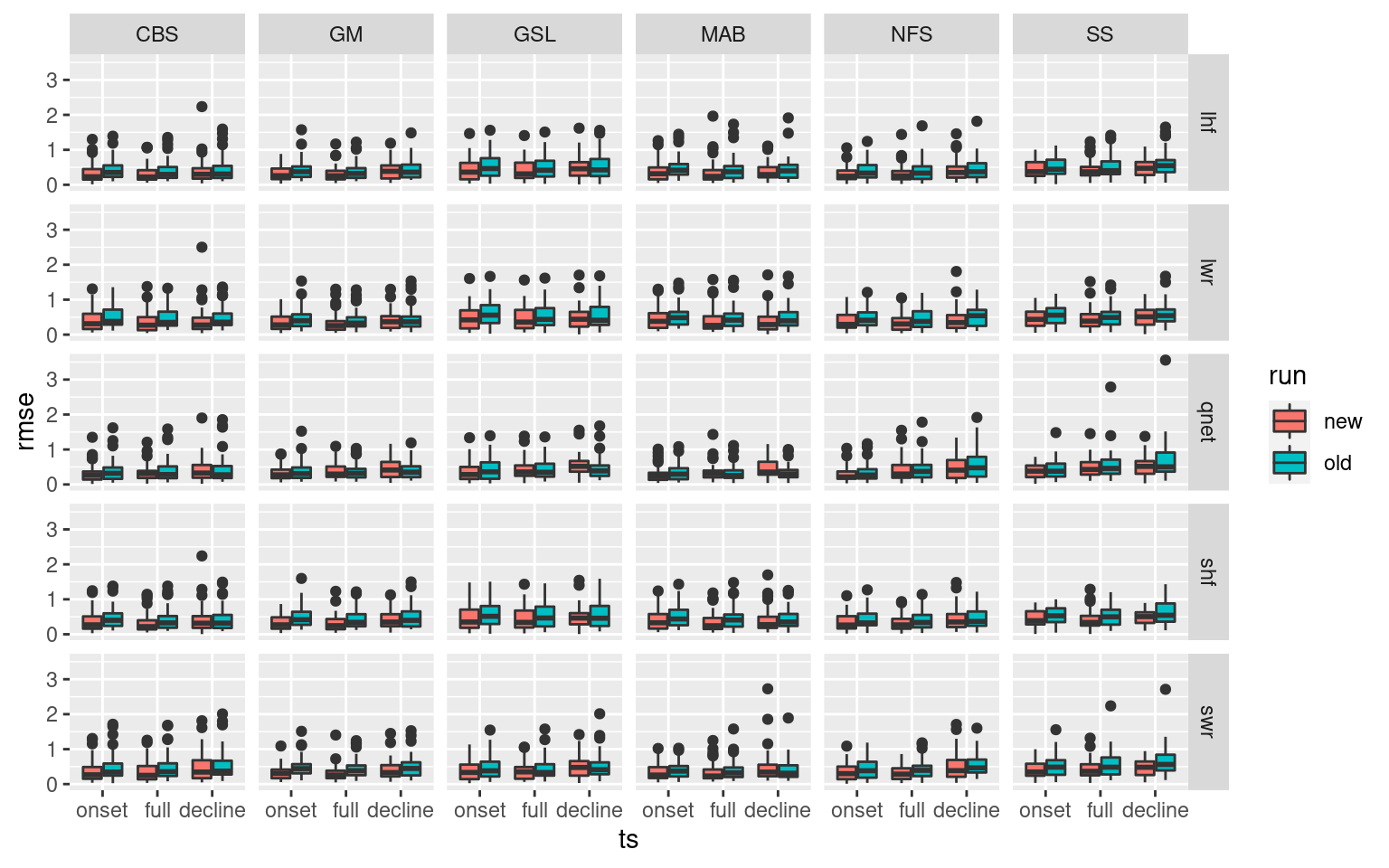
# scale_y_continuous(limits = c(0, 2))The new an improved method that correctly integrates Qx into SSTa creates much lower RMSE values for almost every variable and region. A smashing success.
Small events and the shoaling MLD
An observation was made by one of the reviewers of the manuscript that there appear to be many small MHWs that occur close together. Events that barely peak out above the 90th percentile threshold before dropping back down. More importantly, some of these events appear to be close together in time when doing this, implying that some sort of preconditioning is at play, which was hypothesised to be a continuously shoaled MLD. While we acknowledge that the methods in this manuscript do not attempt to tackle the issue of preconditioning, it is certainly worth investigating the role of the MLD with these MHWs that appear perhaps as a skipping stone, hoping shallowly and rapidly along the curve of the 90th percentile threshold. In the following code we will find these shallow rapid events and relate them to the potential ongoing presence of an anomolously shallow (shoaled) MLD.
# Find the gaps in days between events
dist_days <- function(df){
  res_df <- data.frame()
  for(i in 1:nrow(df)-1){ # A for loop? I know right... is this even tidy code anymore!?
    df_sub <- df[c(i,i+1),]
    df_res <- data.frame(event_1 = df_sub$event_no[1],
                         event_2 = df_sub$event_no[2],
                         days = df_sub$date_start[2] - df_sub$date_end[1])
    res_df <- rbind(res_df, df_res)
  }
  res_df <- na.omit(res_df)
  return(res_df)
}
event_day_dist <- plyr::ddply(OISST_MHW_event, c("region"), dist_days)

# Plot the distribution of differences in days between events
event_day_dist %>%
  group_by(region) %>%
  mutate(count = n()) %>%
  filter(days <= 366) %>% # Let's ignore events more than a year apart
  mutate(count_filter = n()) %>%
  ggplot() +
  geom_histogram(aes(x = as.integer(days), fill = region),
                 bins = 12, show.legend = F) +
  geom_label(aes(x = 200, y = 10, label = paste0(count_filter,"/",count))) +
  facet_wrap(~region)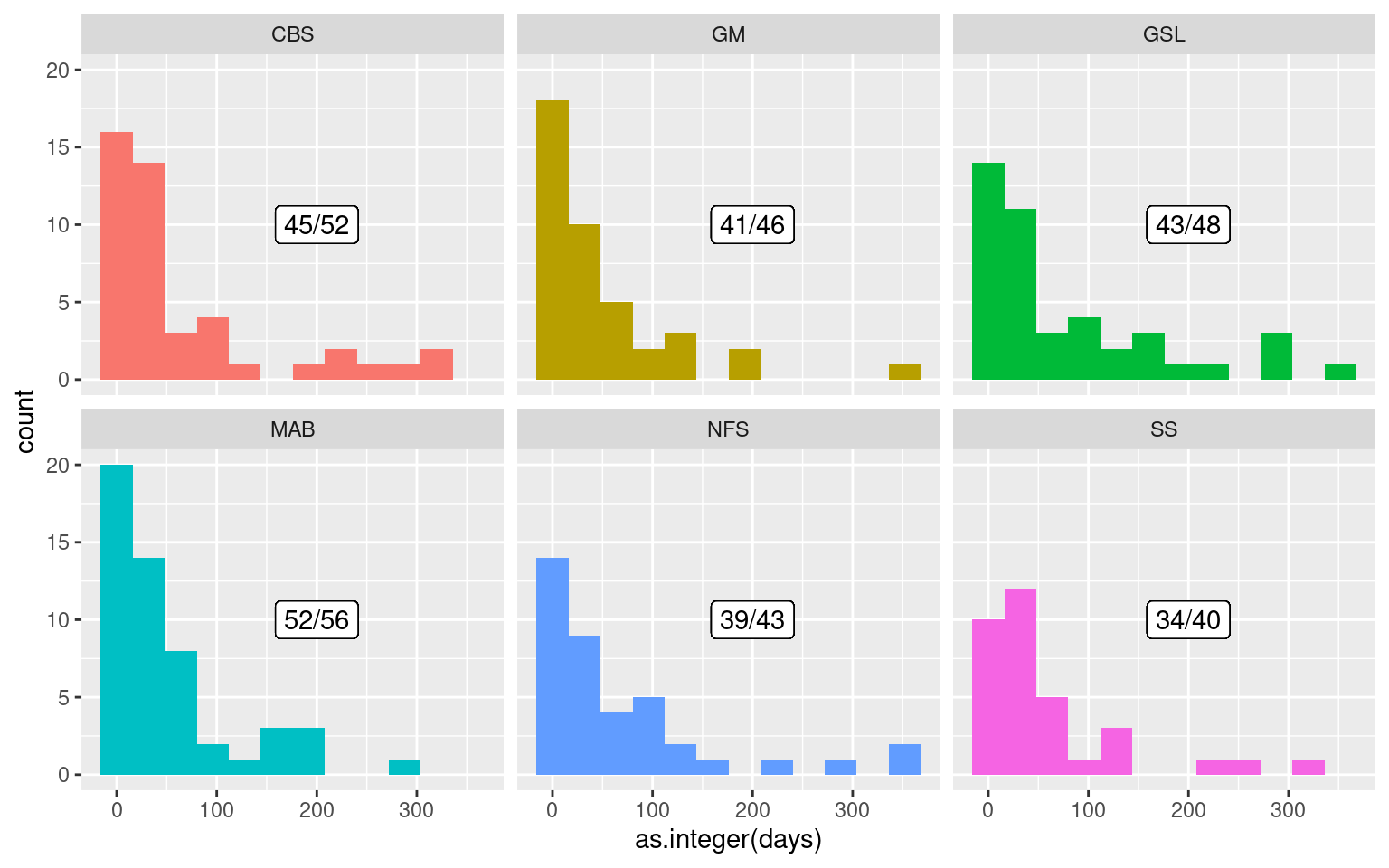
| Version | Author | Date |
|---|---|---|
| 57e2ce3 | robwschlegel | 2021-01-23 |
Of the 291 MHWs detected in the data for this study, 254 of them occur within 366 days of another MHW in the same region. As we may see from the histogram above, most of these events are occurring within two months of another event within the same region. Let’s zoom in on this behaviour and visualise the distribution of gaps between events occurring not more than two months apart.
event_day_dist %>%
  group_by(region) %>%
  mutate(count = n()) %>%
  filter(days <= 62) %>% # Let's ignore events more than a year apart
  mutate(count_filter = n()) %>%
  ggplot() +
  geom_histogram(aes(x = as.integer(days), fill = region),
                 bins = 10, show.legend = F) +
  geom_label(aes(x = 30, y = 5, label = paste0(count_filter,"/",count))) +
  facet_wrap(~region)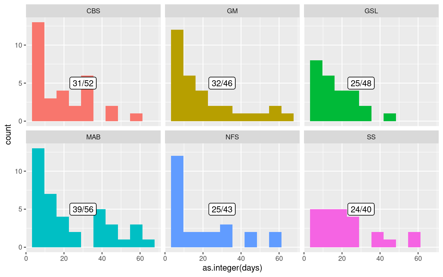
| Version | Author | Date |
|---|---|---|
| 57e2ce3 | robwschlegel | 2021-01-23 |
The above histogram shows us that for the events that are occurring within two months of another month, there is a tendency for the events to occur within one or two weeks of another event. For our main goal here of relating temporally adjacent MHWs to a shoaled MLD we will use a two week filter. This limits the sample to 83 MHWs.
# Subset events
event_day_dist_sub <- event_day_dist %>%
  filter(days <= 14) %>%
  mutate(plyr_idx = 1:n()) # For parallel processing
  # dplyr::select(-days) %>%
  # pivot_longer(event_1:event_2, names_to = "event_no")

# Function for calculating the MLD anomaly between neighbouring MHWs
MLD_neighbour <- function(df){

  # Filter out the two events being compared
  event_1 <- filter(OISST_MHW_event,
                    region == df$region[1], event_no == df$event_1[1])
  event_2 <- filter(OISST_MHW_event,
                    region == df$region[1], event_no == df$event_2[1])

  # Find the dates separating the events
  # We are making a conscious choice to also include the last and first days of the neighbouring events
  # This will account for the ocean state at the very end and beginning of the events
  event_gap <- seq(event_1$date_end, event_2$date_start, by = "day")

  # Extract the MLD data and calculated the cumulative anomaly
  MLD_cum_anom <- filter(ALL_ts_anom, var == "mld",
                         region == df$region[1], t %in% event_gap) %>%
    summarise(count = n(),
              anom_cum = sum(anom),
              anom_mean = mean(anom))

  # Combine and exit
  res <- cbind(df, MLD_cum_anom)
  res$event_1_dur <- event_1$duration[1]
  res$event_2_dur <- event_2$duration[1]
  return(res)
}
MLD_res <- plyr::ddply(event_day_dist_sub, c("plyr_idx"), MLD_neighbour, .parallel = T)
What do the mean and cumulative MLD anomalies look like in the gaps between MHWs occurring within two weeks of each other??
# Cumulative values
hist_cum <- MLD_res %>%
  ggplot() +
  geom_histogram(aes(x = anom_cum, fill = region),
                 bins = 10, show.legend = F) +
  facet_wrap(~region)

# Mean values
hist_mean <- MLD_res %>%
  ggplot() +
  geom_histogram(aes(x = anom_mean, fill = region),
                 bins = 10, show.legend = F) +
  facet_wrap(~region)

# Combine intoa single plot
ggpubr::ggarrange(hist_cum, hist_mean, ncol = 1)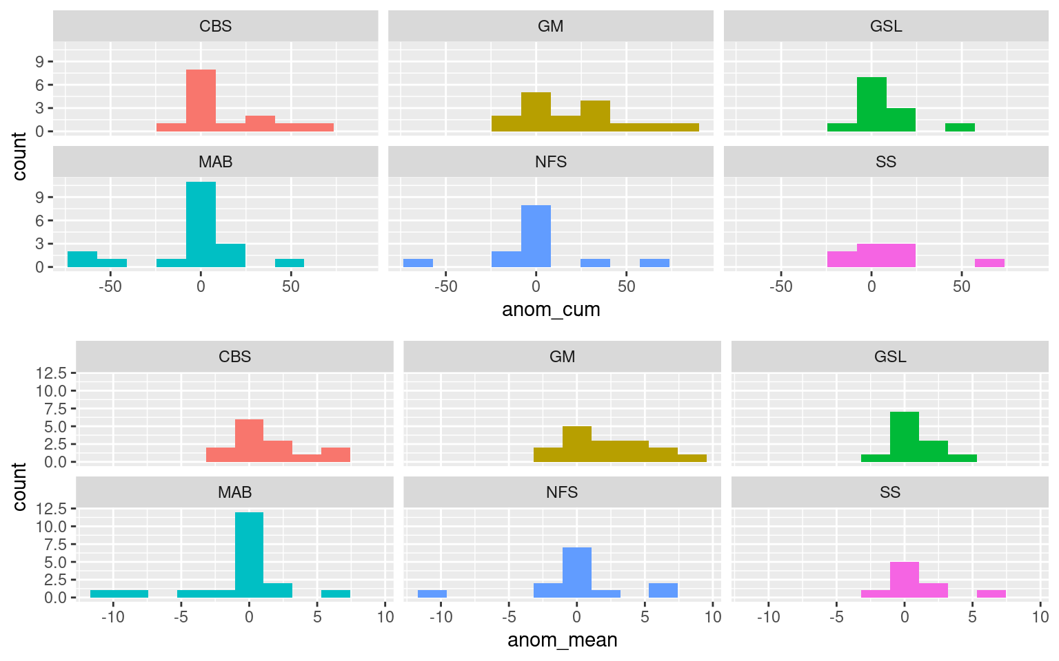
| Version | Author | Date |
|---|---|---|
| 57e2ce3 | robwschlegel | 2021-01-23 |
Above we have plotted histograms of the cumulative and mean MLD anomaly on days between MHWs that occur within two weeks of each other. We have shown the mean values because the cumulative values of events with larger gaps will likely tend to be larger than shorter gaps, even if the MLD may be shoaled more in those gaps. The reader is free to draw their conclusions from either result, but they both show a similar picture, which is that the MLD anomalies during the gaps between nearby MHWs skew towards positive (deeper) depth anomalies. The exception to this being the Mid-Atlantic Bight, and the Newfoundland Shelf to a lesser extent.
Perhaps there is a relationship between the length of the gap and the MLD anomaly?
trend_cum <- MLD_res %>%
  ggplot(aes(x = as.integer(days), y = anom_cum)) +
  geom_point(aes(colour = region)) +
  geom_smooth(method = "lm", se = F, aes(colour = region)) +
  labs(y = "Cumulative anomaly (°C days)", x = "Gap between MHWs (days)")
trend_mean <- MLD_res %>%
  ggplot(aes(x = as.integer(days), y = anom_mean)) +
  geom_point(aes(colour = region)) +
  geom_smooth(method = "lm", se = F, aes(colour = region)) +
  labs(y = "Mean anomaly (°C)", x = "Gap between MHWs (days)")
ggpubr::ggarrange(trend_cum, trend_mean, ncol = 1, common.legend = T)
| Version | Author | Date |
|---|---|---|
| 57e2ce3 | robwschlegel | 2021-01-23 |
Again we’ve shown here the cumulative and mean MLD anomalies during the gapos in events, but this time as dot plots with linear models showing the trend. The standard error of the trends has not been included here because they are so massive. It is very safe to say that none of these trends are significant. There appears to be a bit of a trend in the Gulf of Maine cumulative MLD anomalies with larger gaps between MHWs, but this would be expected by virtue of a larger sample size. The fact that not more of the regions show a trend is what is most interesting. In the mean anomalies we see almost no slope in any regions as the gaps increase or decrease. Looking at the dots in the plot we may see that this is due to the noise in the results.
But this doesn’t quite answer the issue that was posed. Remember that the concern specifically was about very short events occurring close in time to each other. So as a final step we will filter the results from above to only show when two events shorter than 10 days (double the absolute minimum length of five days) occur within two weeks of each other.
MLD_res %>%
  filter(event_1_dur <= 10 & event_2_dur <= 10) %>%
  pivot_longer(anom_cum:anom_mean) %>%
  ggplot() +
  geom_histogram(aes(x = value, fill = region),
                 bins = 10, show.legend = F) +
  facet_grid(region~name, scales = "free_x")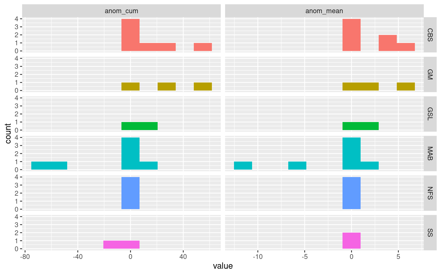
| Version | Author | Date |
|---|---|---|
| 57e2ce3 | robwschlegel | 2021-01-23 |
Now these results are interesting. With the exception of two gaps between adjacent MHWs in the Mid-Atlantic Bight, and one in the Scotian Shelf, the MLD during the gaps between these shallow rapid events is always deeper than seasonally expected, not shallower, as was hypothesised. A possible explanation for this is that these shallow rapid MHWs are actually due to rapidly evolving thermal gradients at the surface. This argument is supported by the fact that of these 25 event pairings, seven of them were recorded in the Mid-Atlantic Bight, and seven were recorded in the Cabot Straight.
Results
Magnitude of change summary
In this sub-section we will look at how the different magnitudes of change for onset and decline of the T_Qnet terms compare to the same changes in SSTa.
# Load magnitude data
ALL_mag <- readRDS("data/ALL_cor.Rda") %>%
  dplyr::select(region:ts, Parameter2, n_Obs, mag) %>%
  na.omit()

# Calculate the proportions of change in magnitudes
ALL_mag_prop <- ALL_mag %>%
  filter(Parameter2 != "sst") %>%
  left_join(filter(ALL_mag, Parameter2 == "sst"),
            by = c("region", "season", "event_no", "ts", "n_Obs")) %>%
  filter(ts != "full") %>%
  dplyr::select(-Parameter2.y) %>%
  dplyr::rename(var = Parameter2.x, mag_Qx = mag.x, mag_SSTa = mag.y) %>%
  mutate(prop = mag_Qx/mag_SSTa) %>%
  mutate(var = as.character(var),
         var = case_when(var == "lwr_budget" ~ "Qlw",
                         var == "swr_budget" ~ "Qsw",
                         var == "lhf_budget" ~ "Qlh",
                         var == "shf_budget" ~ "Qsh",
                         var == "qnet_budget" ~ "Qnet",
                         TRUE ~ var),
         var = factor(var, levels = c("Qnet", "Qlh", "Qsh", "Qlw", "Qsw")),
         region = toupper(region))

# Find an event with good onset and decline match
ALL_mag_prop %>% filter(var == "Qnet", prop >= 1, prop <= 2)
region season event_no ts var n_Obs mag_Qx mag_SSTa prop
1 CBS Winter 2 onset Qnet 20 0.63649297 0.44739441 1.422666
2 CBS Spring 7 onset Qnet 8 0.57527849 0.56663655 1.015251
3 CBS Autumn 9 onset Qnet 11 1.32363504 0.87287571 1.516407
4 CBS Autumn 10 onset Qnet 4 0.61669651 0.34188554 1.803810
5 CBS Summer 11 onset Qnet 15 0.58627169 0.52283736 1.121327
6 CBS Spring 23 onset Qnet 14 1.50567247 0.87550729 1.719771
7 CBS Spring 24 decline Qnet 11 -0.61486410 -0.58549202 1.050166
8 CBS Summer 25 decline Qnet 18 -0.74251689 -0.68569922 1.082861
9 CBS Summer 27 onset Qnet 7 1.01903078 1.01389261 1.005068
10 CBS Summer 27 decline Qnet 18 -1.18218360 -1.07928439 1.095340
11 CBS Autumn 50 onset Qnet 4 0.18317564 0.16876718 1.085375
12 GM Summer 2 onset Qnet 14 1.02631304 0.58907332 1.742250
13 GM Summer 3 onset Qnet 10 0.67764963 0.34956369 1.938558
14 GM Spring 8 onset Qnet 5 0.52867026 0.37336097 1.415976
15 GM Autumn 28 onset Qnet 5 0.62647421 0.33913813 1.847254
16 GM Winter 29 decline Qnet 4 -0.21700063 -0.15318765 1.416567
17 GM Autumn 33 onset Qnet 8 0.27448122 0.25142655 1.091695
18 GM Winter 36 onset Qnet 5 0.22075553 0.16177895 1.364550
19 GM Summer 39 decline Qnet 9 -0.53629652 -0.49158990 1.090943
20 GM Autumn 43 onset Qnet 15 0.55935148 0.53217193 1.051073
21 GM Autumn 44 decline Qnet 4 -0.24527824 -0.23779489 1.031470
22 GM Winter 45 onset Qnet 18 0.74442410 0.38883269 1.914510
23 GSL Summer 3 onset Qnet 5 0.54442864 0.54134207 1.005702
24 GSL Summer 9 onset Qnet 5 0.14784691 0.11522789 1.283083
25 GSL Autumn 10 onset Qnet 3 0.35649717 0.23121691 1.541830
26 GSL Winter 15 onset Qnet 6 0.11259675 0.09486033 1.186974
27 GSL Summer 17 onset Qnet 9 0.42307270 0.32204591 1.313703
28 GSL Winter 21 onset Qnet 32 1.54802506 1.18151078 1.310208
29 GSL Autumn 32 onset Qnet 8 1.02254597 0.95379261 1.072084
30 GSL Autumn 32 decline Qnet 13 -0.83597005 -0.80540865 1.037945
31 GSL Winter 35 onset Qnet 4 0.18358330 0.16318501 1.125001
32 GSL Winter 36 onset Qnet 5 0.09702077 0.07600872 1.276443
33 MAB Autumn 1 onset Qnet 4 0.40452813 0.29639064 1.364848
34 MAB Winter 5 onset Qnet 9 0.51087227 0.35076031 1.456471
35 MAB Summer 7 onset Qnet 3 0.38355752 0.22581522 1.698546
36 MAB Winter 8 decline Qnet 9 -0.87544168 -0.82063566 1.066785
37 MAB Summer 27 onset Qnet 7 0.32998874 0.32811381 1.005714
38 MAB Spring 28 onset Qnet 5 0.58401304 0.33186445 1.759794
39 MAB Summer 30 onset Qnet 6 0.67703554 0.64178920 1.054919
40 MAB Spring 50 onset Qnet 3 0.40339434 0.39490038 1.021509
41 MAB Autumn 51 onset Qnet 3 0.38863084 0.32326054 1.202222
42 MAB Summer 56 onset Qnet 10 1.19591161 0.88742963 1.347613
43 NFS Winter 1 onset Qnet 13 0.53448116 0.52745972 1.013312
44 NFS Spring 3 onset Qnet 17 0.48890672 0.47847078 1.021811
45 NFS Autumn 9 onset Qnet 8 1.02754758 0.91084833 1.128122
46 NFS Spring 11 onset Qnet 5 0.29422076 0.15742727 1.868931
47 NFS Spring 14 onset Qnet 22 1.41299484 1.12830017 1.252322
48 NFS Summer 19 decline Qnet 6 -0.44163771 -0.39255431 1.125036
49 NFS Winter 22 onset Qnet 36 1.10536304 0.65793776 1.680042
50 NFS Winter 24 decline Qnet 4 -0.17600001 -0.17316882 1.016349
51 NFS Winter 27 onset Qnet 7 0.21691586 0.10896060 1.990773
52 NFS Winter 37 onset Qnet 4 0.05434176 0.03863288 1.406619
53 NFS Spring 38 onset Qnet 4 0.50339694 0.31074462 1.619970
54 SS Spring 3 onset Qnet 4 0.55254553 0.38893326 1.420669
55 SS Summer 5 onset Qnet 12 1.22226202 1.15627750 1.057066
56 SS Summer 6 onset Qnet 4 0.51398728 0.42612588 1.206186
57 SS Spring 13 onset Qnet 10 0.95810997 0.80106148 1.196050
58 SS Summer 17 onset Qnet 3 0.49127621 0.48415425 1.014710
59 SS Autumn 26 onset Qnet 3 0.28698888 0.21094822 1.360471
60 SS Summer 35 onset Qnet 4 0.61936000 0.46289489 1.338014
61 SS Summer 37 decline Qnet 6 -0.50665876 -0.37869774 1.337898
62 SS Autumn 38 decline Qnet 49 -2.50176804 -1.55544938 1.608389
63 SS Spring 40 onset Qnet 24 1.46876337 1.40408507 1.046064
64 SS Summer 41 decline Qnet 6 -1.12735714 -1.09602209 1.028590# Create schematic figure showing how magnitudes are calculated
p1 <- fig_mag_func(2, "GSL") +
ggtitle("Good onset, bad decline")
p2 <- fig_mag_func(44, "GM") +
ggtitle("Bad onset, good decline")
p3 <- fig_mag_func(32, "GSL") +
ggtitle("Good onset, good decline")
mag_schematic <- ggpubr::ggarrange(p1, p2, p3, ncol = 3, nrow = 1, common.legend = TRUE)
# mag_schematic
# Scatterplot of SSTa vs SST_Qx (facets per variable)
mag_scatter <- ALL_mag_prop %>%
ggplot(aes(x = mag_SSTa, y = mag_Qx)) +
geom_point(aes(colour = n_Obs, shape = ts)) +
geom_smooth(aes(linetype = ts), method = "lm", colour = "black") +
scale_colour_gradientn(colours = rainbow(10)) +
facet_wrap(~var, nrow = 1) +
labs(x = "ΔSSTa", y = "ΔSST_Qx", shape = "Time series", linetype = "Time series") +
theme(legend.position = "top")
# mag_scatter
# Boxplots of proportions of change for SST_Qx for onset/decline
mag_box <- ALL_mag_prop %>%
ggplot(aes(x = ts, y = prop)) +
geom_hline(aes(yintercept = 0), colour = "red") +
geom_boxplot(aes(fill = season), outlier.shape = NA) +
# geom_boxplot(aes(fill = region), outlier.shape = NA) +
scale_y_continuous(limits = c(-2, 2)) +
facet_wrap(~var, nrow = 1) +
labs(x = NULL, y = "ΔSST_Qx / ΔSSTa")
# mag_box
# Combine for one massive display
mag_full <- ggpubr::ggarrange(mag_schematic, mag_scatter, mag_box, ncol = 1, nrow = 3, labels = c("A)", "B)", "C)"))
ggsave("output/magnitude_schematic.png", height = 8, width = 10)
ggsave("output/magnitude_schematic.pdf", height = 8, width = 10)
mag_full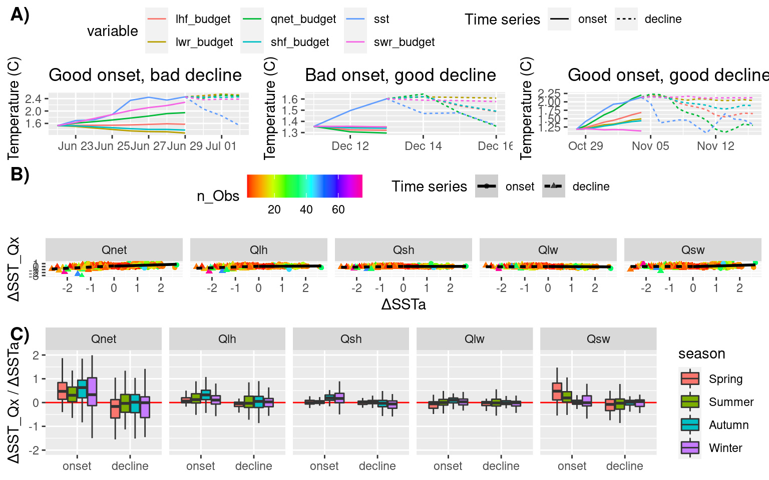
| Version | Author | Date |
|---|---|---|
| a438235 | robwschlegel | 2020-11-10 |
The first thing we want to look at with these magnitude scores is how many MHWs appear to be driven or decayed by Qnet. We determine this if the proportion of change in Qnet is more than half that of the change in SSTa. But also, because the Qx variables can be greater than the sum (Qnet), we will see when individual variables are contributing more than half of the change in SSTa, too.
# Create TRUE/FALSE table when prop is over 0.5 for any variable
ALL_mag_TF <- ALL_mag_prop %>%
  mutate(prop_TF = ifelse(prop > 0.5, TRUE, FALSE)) %>%
  dplyr::select(region:n_Obs, prop_TF) %>%
  pivot_wider(names_from = var, values_from = prop_TF)

# Total proportion of MHWs forced by Qnet
sum(ALL_mag_TF$Qnet)/nrow(ALL_mag_TF)
[1] 0.3319838# Total number of events driven by Qnet
nrow(filter(ALL_mag_TF, ts == "onset", Qnet == TRUE))[1] 122# Total number of events decayed by Qnet
nrow(filter(ALL_mag_TF, ts == "decline", Qnet == TRUE))[1] 42# Proportion of MHWs with Qnet inset and decline
ALL_mag_TF %>%
dplyr::select(region:ts, Qnet) %>%
pivot_wider(names_from = ts, values_from = Qnet) %>%
filter(onset == TRUE, decline == TRUE)# A tibble: 14 x 5
region season event_no onset decline
<chr> <fct> <int> <lgl> <lgl>
1 CBS Spring 24 TRUE TRUE
2 CBS Summer 27 TRUE TRUE
3 CBS Summer 46 TRUE TRUE
4 GSL Winter 15 TRUE TRUE
5 GSL Autumn 32 TRUE TRUE
6 GSL Autumn 46 TRUE TRUE
7 MAB Winter 8 TRUE TRUE
8 MAB Autumn 31 TRUE TRUE
9 MAB Winter 40 TRUE TRUE
10 MAB Autumn 46 TRUE TRUE
11 NFS Autumn 10 TRUE TRUE
12 NFS Winter 22 TRUE TRUE
13 SS Summer 29 TRUE TRUE
14 SS Autumn 38 TRUE TRUE # Counts by time series phase
ALL_mag_count_ts <- ALL_mag_prop %>%
group_by(ts, var) %>%
mutate(ts_count = n(),
group = "Total") %>%
filter(prop > 0.5) %>%
mutate(filter_count = n(),
filter_prop = round(filter_count/ts_count, 2)) %>%
dplyr::select(group, ts, var, filter_prop) %>%
distinct() %>%
mutate(var = factor(var, levels = c("Qnet", "Qlh", "Qsh", "Qlw", "Qsw"))) %>%
pivot_wider(names_from = var, values_from = filter_prop) %>%
dplyr::select(group, ts, Qnet, Qlh, Qsh, Qlw, Qsw)
# knitr::kable(ALL_mag_count_ts)
# Counts by time region phase
ALL_mag_count_region <- ALL_mag_prop %>%
group_by(region, ts, var) %>%
mutate(ts_count = n()) %>%
filter(prop > 0.5) %>%
mutate(filter_count = n(),
filter_prop = round(filter_count/ts_count, 2)) %>%
dplyr::select(region, ts, var, filter_prop) %>%
distinct() %>%
pivot_wider(names_from = var, values_from = filter_prop) %>%
dplyr::select(region, ts, Qnet, Qlh, Qsh, Qlw, Qsw) %>%
arrange(region, ts) %>%
dplyr::rename(group = region)
# knitr::kable(ALL_mag_count_region)
# Counts by time series phase
ALL_mag_count_season <- ALL_mag_prop %>%
group_by(season, ts, var) %>%
mutate(ts_count = n()) %>%
filter(prop > 0.5) %>%
mutate(filter_count = n(),
filter_prop = round(filter_count/ts_count, 2)) %>%
dplyr::select(season, ts, var, filter_prop) %>%
distinct() %>%
pivot_wider(names_from = var, values_from = filter_prop) %>%
dplyr::select(season, ts, Qnet, Qlh, Qsh, Qlw, Qsw) %>%
arrange(season, ts) %>%
dplyr::rename(group = season)
# knitr::kable(ALL_mag_count_season)
ALL_mag_count_ts_region_season <- rbind(ALL_mag_count_ts, ALL_mag_count_region, ALL_mag_count_season) %>%
dplyr::select(group:Qnet) %>%
pivot_wider(names_from = ts, values_from = Qnet) %>%
dplyr::select(group, onset, decline) %>%
mutate(onset = paste0(onset*100,"%"),
decline = paste0(decline*100,"%"))
knitr::kable(ALL_mag_count_ts_region_season)| group | onset | decline |
|---|---|---|
| Total | 49% | 17% |
| CBS | 49% | 16% |
| GM | 49% | 16% |
| GSL | 43% | 10% |
| MAB | 56% | 14% |
| NFS | 57% | 19% |
| SS | 36% | 32% |
| Spring | 51% | 7% |
| Summer | 40% | 20% |
| Autumn | 61% | 18% |
| Winter | 46% | 20% |
We also want a table showing the count of best magnitude match per variable per region/season.
# Get the top results other than Qnet
ALL_mag_top <- ALL_mag_prop %>%
  filter(var != "Qnet") %>% # Remove Qnet
  group_by(region, season, event_no, ts) %>%
  filter(prop == max(prop))

# The top count by region
ALL_mag_region <- ALL_mag_top %>%
  group_by(region, ts, var) %>%
  summarise(count = n(), .groups = "drop") %>%
  pivot_wider(names_from = var, values_from = count) %>%
  mutate(Qlw = replace_na(Qlw, 0)) %>%
  left_join(count_region, by = c("region", "ts")) %>%
  dplyr::select(region, ts, count, Qlh:Qsw) %>%
  mutate(Qlh = paste0(Qlh, " (",round((Qlh/count)*100),"%)"),
         Qsh = paste0(Qsh, " (",round((Qsh/count)*100),"%)"),
         Qlw = paste0(Qlw, " (",round((Qlw/count)*100),"%)"),
         Qsw = paste0(Qsw, " (",round((Qsw/count)*100),"%)")) %>%
  dplyr::rename(group = region)
# knitr::kable(ALL_mag_region)

# The top count by season
ALL_mag_season <- ALL_mag_top %>%
  group_by(season, ts, var) %>%
  summarise(count = n(), .groups = "drop") %>%
  pivot_wider(names_from = var, values_from = count) %>%
  mutate(Qsh = replace_na(Qsh, 0)) %>%
  left_join(count_season, by = c("season", "ts")) %>%
  dplyr::select(season, ts, count, Qlh:Qsw) %>%
  mutate(Qlh = paste0(Qlh, " (",round((Qlh/count)*100),"%)"),
         Qsh = paste0(Qsh, " (",round((Qsh/count)*100),"%)"),
         Qlw = paste0(Qlw, " (",round((Qlw/count)*100),"%)"),
         Qsw = paste0(Qsw, " (",round((Qsw/count)*100),"%)")) %>%
  dplyr::rename(group = season)
# knitr::kable(ALL_mag_season)

# Print table
ALL_mag_region_season <- rbind(ALL_mag_region, ALL_mag_season)
knitr::kable(ALL_mag_region_season)| group | ts | count | Qlh | Qsh | Qlw | Qsw |
|---|---|---|---|---|---|---|
| CBS | onset | 43 | 12 (28%) | 10 (23%) | 6 (14%) | 15 (35%) |
| CBS | decline | 43 | 10 (23%) | 3 (7%) | 14 (33%) | 16 (37%) |
| GM | onset | 41 | 9 (22%) | 5 (12%) | 9 (22%) | 18 (44%) |
| GM | decline | 38 | 12 (32%) | 3 (8%) | 5 (13%) | 18 (47%) |
| GSL | onset | 44 | 13 (30%) | 4 (9%) | 4 (9%) | 23 (52%) |
| GSL | decline | 41 | 9 (22%) | 6 (15%) | 10 (24%) | 16 (39%) |
| MAB | onset | 50 | 18 (36%) | 8 (16%) | 0 (0%) | 24 (48%) |
| MAB | decline | 50 | 15 (30%) | 8 (16%) | 15 (30%) | 12 (24%) |
| NFS | onset | 37 | 14 (38%) | 3 (8%) | 6 (16%) | 14 (38%) |
| NFS | decline | 37 | 10 (27%) | 2 (5%) | 14 (38%) | 11 (30%) |
| SS | onset | 36 | 9 (25%) | 2 (6%) | 8 (22%) | 17 (47%) |
| SS | decline | 34 | 11 (32%) | 2 (6%) | 6 (18%) | 15 (44%) |
| Spring | onset | 53 | 5 (9%) | 1 (2%) | 7 (13%) | 40 (75%) |
| Spring | decline | 42 | 6 (14%) | 10 (24%) | 11 (26%) | 15 (36%) |
| Summer | onset | 88 | 28 (32%) | 0 (0%) | 8 (9%) | 52 (59%) |
| Summer | decline | 88 | 22 (25%) | 7 (8%) | 27 (31%) | 32 (36%) |
| Autumn | onset | 62 | 38 (61%) | 11 (18%) | 6 (10%) | 7 (11%) |
| Autumn | decline | 62 | 26 (42%) | 0 (0%) | 16 (26%) | 20 (32%) |
| Winter | onset | 48 | 4 (8%) | 20 (42%) | 12 (25%) | 12 (25%) |
| Winter | decline | 51 | 13 (25%) | 7 (14%) | 10 (20%) | 21 (41%) |
These tables help to reiterate how much more important Qlh is for the onset and decline of MHWs over the other variables, and that Qsw often comes in second. For the seasons though we see a much more complex relationship that I won’t go into here.
RMSE summary
Here we will go about summarising the RMSE results. We will also create some boxplots to help with the process.
# The base RMSE results
ALL_RMSE <- ALL_cor %>%
  filter(rmse > 0 ) %>%
  dplyr::rename(var = Parameter2) %>%
  dplyr::select(region:ts, var, n_Obs, rmse) %>%
  mutate(var = as.character(var),
         var = case_when(var == "lwr_budget" ~ "Qlw",
                         var == "swr_budget" ~ "Qsw",
                         var == "lhf_budget" ~ "Qlh",
                         var == "shf_budget" ~ "Qsh",
                         var == "qnet_budget" ~ "Qnet",
                         TRUE ~ var),
         var = factor(var, levels = c("Qnet", "Qlh", "Qsh", "Qlw", "Qsw")),
         region = toupper(region)) %>%
  # filter out events where Qnet is not a primary drivers
  left_join(ALL_mag_TF, by = c("region", "season", "event_no", "ts", "n_Obs")) %>%
  filter(Qnet == TRUE)

# Summaries by region
ALL_RMSE_region <- ALL_RMSE %>%
  dplyr::select(-season, -event_no, -n_Obs) %>%
  group_by(region, ts, var) %>%
  summarise(rmse_min = min(rmse),
           rmse_mean = mean(rmse),
           rmse_max = max(rmse), .groups = "drop")

# Boxplot of region summaries
ALL_RMSE %>%
  dplyr::select(-season, -event_no, -n_Obs) %>%
  ggplot(aes(x = var, y = rmse)) +
  geom_boxplot(aes(fill = ts)) +
  facet_wrap(~region) #+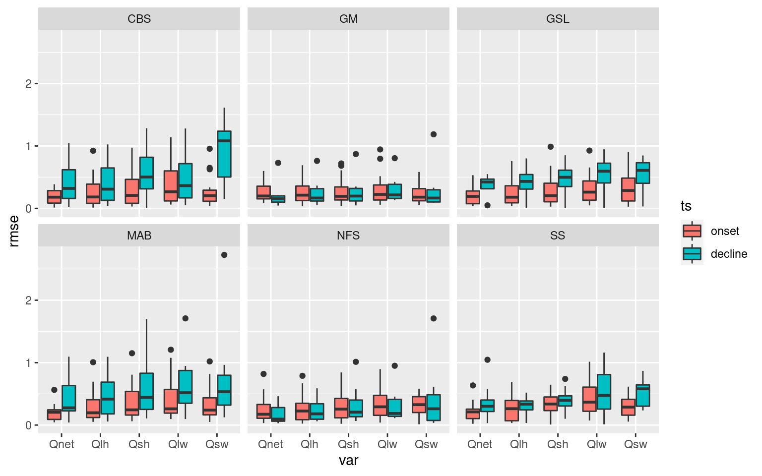
  # theme(axis.text.x = element_text(angle = 45))

# Summaries by season
ALL_RMSE_season <- ALL_RMSE %>%
  dplyr::select(-region, -event_no, -n_Obs) %>%
  group_by(season, ts, var) %>%
  summarise(rmse_min = min(rmse),
           rmse_mean = mean(rmse),
           rmse_max = max(rmse), .groups = "drop")

# Boxplot of season results
ALL_RMSE %>%
  dplyr::select(-region, -event_no, -n_Obs) %>%
  ggplot(aes(x = var, y = rmse)) +
  geom_boxplot(aes(fill = ts)) +
  facet_wrap(~season)
# Boxplot by variable
ALL_RMSE %>%
  filter(var != "Qnet") %>%
  ggplot(aes(x = region, y = rmse)) +
  geom_boxplot(aes(fill = ts)) +
  facet_wrap(~var)
| Version | Author | Date |
|---|---|---|
| a438235 | robwschlegel | 2020-11-10 |
ALL_RMSE %>%
    filter(var != "Qnet") %>%
  ggplot(aes(x = season, y = rmse)) +
  geom_boxplot(aes(fill = ts)) +
  facet_wrap(~var)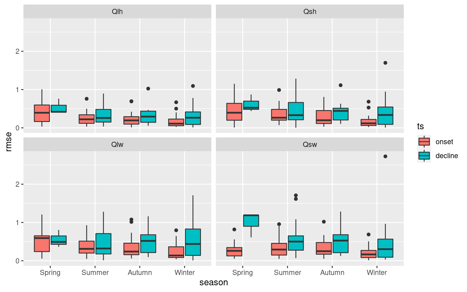
| Version | Author | Date |
|---|---|---|
| a438235 | robwschlegel | 2020-11-10 |
These boxplots help to tell a high level story about the importance of the Qx variables with SSTa, but I want a slightly more fine-grain level of results. To do this I am going to count which of the Qx variables has the lowest RMSE per MHW. These will then be grouped by region and season to provide an understanding for how this may vary.
# Get the top results other than Qnet
ALL_RMSE_top <- ALL_RMSE %>%
  filter(var != "Qnet") %>% # Remove Qnet
  group_by(region, season, event_no, ts) %>%
  filter(rmse == min(rmse))

# The top count overall
ALL_RMSE_ts <- ALL_RMSE_top %>%
  group_by(ts) %>%
  mutate(total_count = n(),
         group = "Total") %>%
  group_by(group, ts, total_count, var) %>%
  summarise(count = n(), .groups = "drop") %>%
  pivot_wider(names_from = var, values_from = count) %>%
  replace_na(list(Qlh = 0, Qsh = 0, Qlw = 0, Qsw = 0)) %>%
  dplyr::select(group, ts, total_count, Qlh:Qsw) %>%
  filter(ts != "full") %>%
  mutate(Qlh = paste0(Qlh, " (",round((Qlh/total_count)*100),"%)"),
         Qsh = paste0(Qsh, " (",round((Qsh/total_count)*100),"%)"),
         Qlw = paste0(Qlw, " (",round((Qlw/total_count)*100),"%)"),
         Qsw = paste0(Qsw, " (",round((Qsw/total_count)*100),"%)"))

# The top count by region
ALL_RMSE_region <- ALL_RMSE_top %>%
  group_by(region, ts) %>%
  mutate(total_count = n()) %>%
  group_by(region, ts, total_count, var) %>%
  summarise(count = n(), .groups = "drop") %>%
  pivot_wider(names_from = var, values_from = count) %>%
  replace_na(list(Qlh = 0, Qsh = 0, Qlw = 0, Qsw = 0)) %>%
  dplyr::select(region, ts, total_count, Qlh:Qlw) %>%
  filter(ts != "full") %>%
  mutate(Qlh = paste0(Qlh, " (",round((Qlh/total_count)*100),"%)"),
         Qsh = paste0(Qsh, " (",round((Qsh/total_count)*100),"%)"),
         Qlw = paste0(Qlw, " (",round((Qlw/total_count)*100),"%)"),
         Qsw = paste0(Qsw, " (",round((Qsw/total_count)*100),"%)")) %>%
  dplyr::rename(group = region)
# knitr::kable(ALL_RMSE_region)

# The top count by season
ALL_RMSE_season <- ALL_RMSE_top %>%
  group_by(season, ts) %>%
  mutate(total_count = n()) %>%
  group_by(season, ts, total_count, var) %>%
  summarise(count = n(), .groups = "drop") %>%
  pivot_wider(names_from = var, values_from = count) %>%
  replace_na(list(Qlh = 0, Qsh = 0, Qlw = 0, Qsw = 0)) %>%
  dplyr::select(season, ts, total_count, Qlh:Qlw) %>%
  filter(ts != "full") %>%
  mutate(Qlh = paste0(Qlh, " (",round((Qlh/total_count)*100),"%)"),
         Qsh = paste0(Qsh, " (",round((Qsh/total_count)*100),"%)"),
         Qlw = paste0(Qlw, " (",round((Qlw/total_count)*100),"%)"),
         Qsw = paste0(Qsw, " (",round((Qsw/total_count)*100),"%)")) %>%
  dplyr::rename(group = season)
# knitr::kable(ALL_RMSE_season)

# Print table
ALL_RMSE_ts_region_season <- rbind(ALL_RMSE_ts, ALL_RMSE_region, ALL_RMSE_season) %>%
  dplyr::rename(count = total_count)
knitr::kable(ALL_RMSE_ts_region_season)| group | ts | count | Qlh | Qsh | Qlw | Qsw |
|---|---|---|---|---|---|---|
| Total | onset | 122 | 57 (47%) | 22 (18%) | 2 (2%) | 41 (34%) |
| Total | decline | 42 | 26 (62%) | 3 (7%) | 6 (14%) | 7 (17%) |
| CBS | onset | 21 | 9 (43%) | 3 (14%) | 0 (0%) | 9 (43%) |
| CBS | decline | 7 | 2 (29%) | 1 (14%) | 4 (57%) | 0 (0%) |
| GM | onset | 20 | 6 (30%) | 4 (20%) | 1 (5%) | 9 (45%) |
| GM | decline | 6 | 3 (50%) | 1 (17%) | 0 (0%) | 2 (33%) |
| GSL | onset | 19 | 10 (53%) | 3 (16%) | 1 (5%) | 5 (26%) |
| GSL | decline | 4 | 3 (75%) | 1 (25%) | 0 (0%) | 0 (0%) |
| MAB | onset | 28 | 14 (50%) | 6 (21%) | 0 (0%) | 8 (29%) |
| MAB | decline | 7 | 7 (100%) | 0 (0%) | 0 (0%) | 0 (0%) |
| NFS | onset | 21 | 11 (52%) | 5 (24%) | 0 (0%) | 5 (24%) |
| NFS | decline | 7 | 5 (71%) | 0 (0%) | 0 (0%) | 2 (29%) |
| SS | onset | 13 | 7 (54%) | 1 (8%) | 0 (0%) | 5 (38%) |
| SS | decline | 11 | 6 (55%) | 0 (0%) | 2 (18%) | 3 (27%) |
| Spring | onset | 27 | 7 (26%) | 3 (11%) | 0 (0%) | 17 (63%) |
| Spring | decline | 3 | 2 (67%) | 0 (0%) | 1 (33%) | 0 (0%) |
| Summer | onset | 35 | 20 (57%) | 2 (6%) | 0 (0%) | 13 (37%) |
| Summer | decline | 18 | 10 (56%) | 1 (6%) | 4 (22%) | 3 (17%) |
| Autumn | onset | 38 | 24 (63%) | 9 (24%) | 1 (3%) | 4 (11%) |
| Autumn | decline | 11 | 10 (91%) | 0 (0%) | 1 (9%) | 0 (0%) |
| Winter | onset | 22 | 6 (27%) | 8 (36%) | 1 (5%) | 7 (32%) |
| Winter | decline | 10 | 4 (40%) | 2 (20%) | 0 (0%) | 4 (40%) |
I’m pretty happy with how these results are displayed. In the last chunk in this sub-section we will grab some specific summary stats that are used in the publication.
# Short event best fits
ALL_RMSE_short <- ALL_RMSE %>%
  filter(n_Obs <= 14, var != "Qnet") %>%
  group_by(region, season, event_no, ts) %>%
  filter(rmse == min(rmse))

# Short event index
ALL_RMSE_long <- ALL_RMSE %>%
  filter(n_Obs > 14, var != "Qnet") %>%
  group_by(region, season, event_no, ts) %>%
  filter(rmse == min(rmse))

# The top Qx for events of 14 days or less by region
ALL_RMSE_short_region <- ALL_RMSE_short %>%
  group_by(region, ts) %>%
  mutate(count = n()) %>%
  group_by(region, ts, count, var) %>%
  summarise(count_Q = n(), .groups = "drop") %>%
  pivot_wider(names_from = var, values_from = count_Q) %>%
  replace_na(list(Qlh = 0, Qsh = 0, Qlw = 0, Qsw = 0)) %>%
  dplyr::select(region, ts, count, Qlh:Qlw) %>%
  mutate(Qlh = paste0(Qlh, " (",round((Qlh/count)*100),"%)"),
         Qsh = paste0(Qsh, " (",round((Qsh/count)*100),"%)"),
         Qlw = paste0(Qlw, " (",round((Qlw/count)*100),"%)"),
         Qsw = paste0(Qsw, " (",round((Qsw/count)*100),"%)"))
knitr::kable(ALL_RMSE_short_region)| region | ts | count | Qlh | Qsh | Qsw | Qlw |
|---|---|---|---|---|---|---|
| CBS | onset | 18 | 7 (39%) | 3 (17%) | 8 (44%) | 0 (0%) |
| CBS | decline | 4 | 1 (25%) | 1 (25%) | 0 (0%) | 2 (50%) |
| GM | onset | 16 | 4 (25%) | 3 (19%) | 9 (56%) | 0 (0%) |
| GM | decline | 5 | 2 (40%) | 1 (20%) | 2 (40%) | 0 (0%) |
| GSL | onset | 17 | 10 (59%) | 2 (12%) | 4 (24%) | 1 (6%) |
| GSL | decline | 3 | 2 (67%) | 1 (33%) | 0 (0%) | 0 (0%) |
| MAB | onset | 24 | 12 (50%) | 4 (17%) | 8 (33%) | 0 (0%) |
| MAB | decline | 3 | 3 (100%) | 0 (0%) | 0 (0%) | 0 (0%) |
| NFS | onset | 17 | 8 (47%) | 4 (24%) | 5 (29%) | 0 (0%) |
| NFS | decline | 5 | 3 (60%) | 0 (0%) | 2 (40%) | 0 (0%) |
| SS | onset | 10 | 6 (60%) | 1 (10%) | 3 (30%) | 0 (0%) |
| SS | decline | 7 | 4 (57%) | 0 (0%) | 1 (14%) | 2 (29%) |
# The top Qx for events of more than 14 days by region
ALL_RMSE_long_region <- ALL_RMSE_long %>%
  group_by(region, ts) %>%
  mutate(count = n()) %>%
  group_by(region, ts, count, var) %>%
  summarise(count_Q = n(), .groups = "drop") %>%
  pivot_wider(names_from = var, values_from = count_Q) %>%
  replace_na(list(Qlh = 0, Qsh = 0, Qlw = 0, Qsw = 0)) %>%
  dplyr::select(region, ts, count, Qlh:Qsh) %>%
  mutate(Qlh = paste0(Qlh, " (",round((Qlh/count)*100),"%)"),
         Qsh = paste0(Qsh, " (",round((Qsh/count)*100),"%)"),
         Qlw = paste0(Qlw, " (",round((Qlw/count)*100),"%)"),
         Qsw = paste0(Qsw, " (",round((Qsw/count)*100),"%)"))
knitr::kable(ALL_RMSE_long_region)| region | ts | count | Qlh | Qsw | Qlw | Qsh |
|---|---|---|---|---|---|---|
| CBS | onset | 3 | 2 (67%) | 1 (33%) | 0 (0%) | 0 (0%) |
| CBS | decline | 3 | 1 (33%) | 0 (0%) | 2 (67%) | 0 (0%) |
| GM | onset | 4 | 2 (50%) | 0 (0%) | 1 (25%) | 1 (25%) |
| GM | decline | 1 | 1 (100%) | 0 (0%) | 0 (0%) | 0 (0%) |
| GSL | onset | 2 | 0 (0%) | 1 (50%) | 0 (0%) | 1 (50%) |
| GSL | decline | 1 | 1 (100%) | 0 (0%) | 0 (0%) | 0 (0%) |
| MAB | onset | 4 | 2 (50%) | 0 (0%) | 0 (0%) | 2 (50%) |
| MAB | decline | 4 | 4 (100%) | 0 (0%) | 0 (0%) | 0 (0%) |
| NFS | onset | 4 | 3 (75%) | 0 (0%) | 0 (0%) | 1 (25%) |
| NFS | decline | 2 | 2 (100%) | 0 (0%) | 0 (0%) | 0 (0%) |
| SS | onset | 3 | 1 (33%) | 2 (67%) | 0 (0%) | 0 (0%) |
| SS | decline | 4 | 2 (50%) | 2 (50%) | 0 (0%) | 0 (0%) |
# The top Qx for events of 14 days or less by season
ALL_RMSE_short_season <- ALL_RMSE_short %>%
  group_by(season, ts) %>%
  mutate(count = n()) %>%
  group_by(season, ts, count, var) %>%
  summarise(count_Q = n(), .groups = "drop") %>%
  pivot_wider(names_from = var, values_from = count_Q) %>%
  replace_na(list(Qlh = 0, Qsh = 0, Qlw = 0, Qsw = 0)) %>%
  dplyr::select(season, ts, count, Qlh:Qlw) %>%
  mutate(Qlh = paste0(Qlh, " (",round((Qlh/count)*100),"%)"),
         Qsh = paste0(Qsh, " (",round((Qsh/count)*100),"%)"),
         Qlw = paste0(Qlw, " (",round((Qlw/count)*100),"%)"),
         Qsw = paste0(Qsw, " (",round((Qsw/count)*100),"%)"))
knitr::kable(ALL_RMSE_short_season)| season | ts | count | Qlh | Qsh | Qsw | Qlw |
|---|---|---|---|---|---|---|
| Spring | onset | 22 | 6 (27%) | 2 (9%) | 14 (64%) | 0 (0%) |
| Spring | decline | 1 | 0 (0%) | 0 (0%) | 0 (0%) | 1 (100%) |
| Summer | onset | 33 | 18 (55%) | 2 (6%) | 13 (39%) | 0 (0%) |
| Summer | decline | 14 | 7 (50%) | 1 (7%) | 3 (21%) | 3 (21%) |
| Autumn | onset | 29 | 19 (66%) | 6 (21%) | 3 (10%) | 1 (3%) |
| Autumn | decline | 7 | 7 (100%) | 0 (0%) | 0 (0%) | 0 (0%) |
| Winter | onset | 18 | 4 (22%) | 7 (39%) | 7 (39%) | 0 (0%) |
| Winter | decline | 5 | 1 (20%) | 2 (40%) | 2 (40%) | 0 (0%) |
# The top Qx for events of more than 14 days by season
ALL_RMSE_long_season <- ALL_RMSE_long %>%
  group_by(season, ts) %>%
  mutate(count = n()) %>%
  group_by(season, ts, count, var) %>%
  summarise(count_Q = n(), .groups = "drop") %>%
  pivot_wider(names_from = var, values_from = count_Q) %>%
  replace_na(list(Qlh = 0, Qsh = 0, Qlw = 0, Qsw = 0)) %>%
  dplyr::select(season, ts, count, Qlh:Qlw) %>%
  mutate(Qlh = paste0(Qlh, " (",round((Qlh/count)*100),"%)"),
         Qsh = paste0(Qsh, " (",round((Qsh/count)*100),"%)"),
         Qlw = paste0(Qlw, " (",round((Qlw/count)*100),"%)"),
         Qsw = paste0(Qsw, " (",round((Qsw/count)*100),"%)"))
knitr::kable(ALL_RMSE_long_season)| season | ts | count | Qlh | Qsh | Qsw | Qlw |
|---|---|---|---|---|---|---|
| Spring | onset | 5 | 1 (20%) | 1 (20%) | 3 (60%) | 0 (0%) |
| Spring | decline | 2 | 2 (100%) | 0 (0%) | 0 (0%) | 0 (0%) |
| Summer | onset | 2 | 2 (100%) | 0 (0%) | 0 (0%) | 0 (0%) |
| Summer | decline | 4 | 3 (75%) | 0 (0%) | 0 (0%) | 1 (25%) |
| Autumn | onset | 9 | 5 (56%) | 3 (33%) | 1 (11%) | 0 (0%) |
| Autumn | decline | 4 | 3 (75%) | 0 (0%) | 0 (0%) | 1 (25%) |
| Winter | onset | 4 | 2 (50%) | 1 (25%) | 0 (0%) | 1 (25%) |
| Winter | decline | 5 | 3 (60%) | 0 (0%) | 2 (40%) | 0 (0%) |
We also want to see how RMSE scores change the shorter the phase of the MHW is.
# Faceted scatter plot showing how RMSE changes based on ts length
ggplot(ALL_RMSE, aes(x = n_Obs, y = rmse)) +
  geom_point(aes(colour = ts)) +
  geom_smooth(aes(colour = ts), method = "lm") +
  facet_wrap(~region)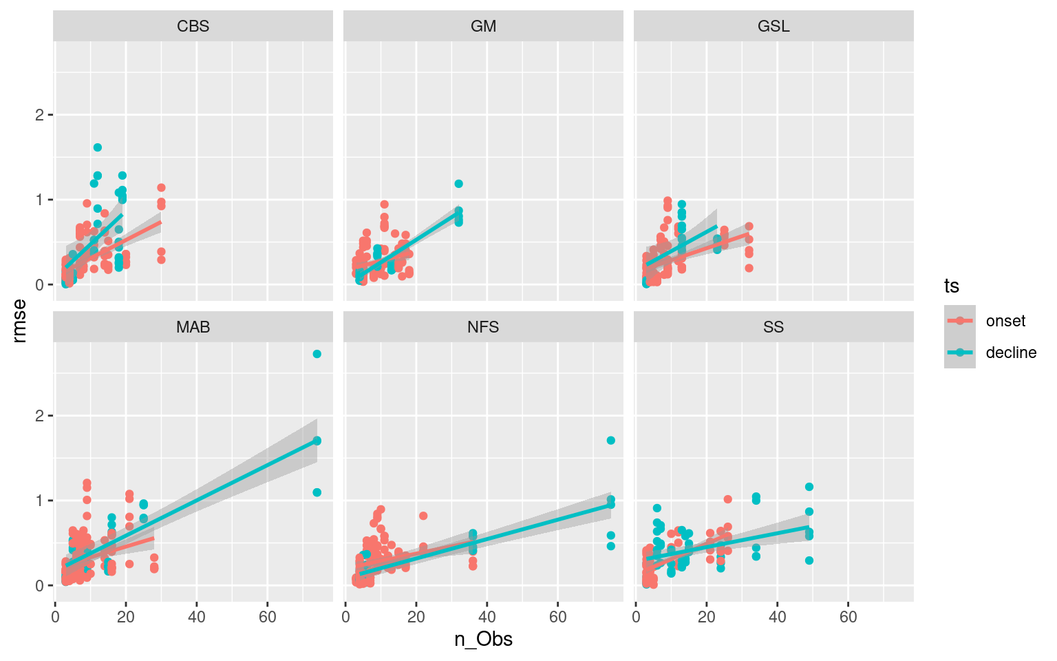
# Faceted scatter plot showing how RMSE changes based on ts length
ggplot(ALL_RMSE, aes(x = n_Obs, y = rmse)) +
  geom_point(aes(colour = ts)) +
  geom_smooth(aes(colour = ts), method = "lm") +
  facet_wrap(~season)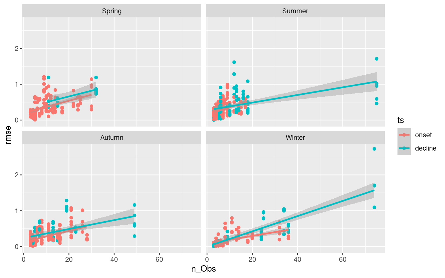
Correlations: summary, regions, seasons
With the correlations calculated for the onset, decline, and full extent of each MHW, we want to know if any signals emerge from the regions and/or seasons of occurrence of these events. Is the relationship between SSS and MHW onset stronger in the winter? Stronger in certain region? Having manually looked through the shiny app it does look like there are some patterns. Below is the code used to determine the stats referred to in the paper.
# Overall correlation results
cor_summary_all <- ALL_cor %>%
  filter(Parameter1 == "sst",
         Parameter2 != "sst") %>%
  group_by(ts, Parameter2) %>%
  summarise(q10_r = quantile(r, 0.1),
            mean_r = mean(r, na.rm = T),
            q90_r = quantile(r, 0.9),
            mean_rmse = mean(rmse, na.rm = T))

# Overall positive only results
cor_positive_all <- ALL_cor %>%
  filter(Parameter1 == "sst",
         Parameter2 != "sst",
         r > 0) %>%
  group_by(ts, Parameter2) %>%
  summarise(q10_r = quantile(r, 0.1),
            mean_r = mean(r, na.rm = T),
            q90_r = quantile(r, 0.9),
            mean_rmse = mean(rmse, na.rm = T))

# Overall negative only results
cor_negative_all <- ALL_cor %>%
  filter(Parameter1 == "sst",
         Parameter2 != "sst",
         r < 0) %>%
  group_by(ts, Parameter2) %>%
  summarise(q10_r = quantile(r, 0.1),
            mean_r = mean(r, na.rm = T),
            q90_r = quantile(r, 0.9),
            mean_rmse = mean(rmse, na.rm = T))

# region correlation results
cor_summary_region <- ALL_cor %>%
  filter(Parameter1 == "sst",
         Parameter2 != "sst") %>%
  group_by(ts, region, Parameter2) %>%
  summarise(q10_r = quantile(r, 0.1),
            mean_r = mean(r, na.rm = T),
            q90_r = quantile(r, 0.9),
            mean_rmse = mean(rmse, na.rm = T))

# Look at specific results
cor_summary_region %>%
  filter(Parameter2 == "mld_cum")
# A tibble: 18 x 7
# Groups: ts, region [18]
ts region Parameter2 q10_r mean_r q90_r mean_rmse
<fct> <chr> <fct> <dbl> <dbl> <dbl> <dbl>
1 onset CBS mld_cum -0.986 -0.578 0.39 NaN
2 onset GM mld_cum -0.96 -0.413 0.74 NaN
3 onset GSL mld_cum -0.99 -0.641 0.396 NaN
4 onset MAB mld_cum -0.981 -0.784 -0.595 NaN
5 onset NFS mld_cum -0.97 -0.652 -0.182 NaN
6 onset SS mld_cum -0.98 -0.584 0.535 NaN
7 full CBS mld_cum -0.76 -0.0602 0.568 NaN
8 full GM mld_cum -0.676 -0.0589 0.704 NaN
9 full GSL mld_cum -0.762 -0.170 0.356 NaN
10 full MAB mld_cum -0.774 -0.225 0.416 NaN
11 full NFS mld_cum -0.79 -0.0909 0.567 NaN
12 full SS mld_cum -0.79 -0.153 0.54 NaN
13 decline CBS mld_cum -0.85 0.400 0.976 NaN
14 decline GM mld_cum -0.916 0.247 0.94 NaN
15 decline GSL mld_cum -0.86 0.517 0.98 NaN
16 decline MAB mld_cum -0.671 0.358 0.99 NaN
17 decline NFS mld_cum -0.67 0.517 0.974 NaN
18 decline SS mld_cum -0.797 0.227 0.99 NaN# region correlation results
cor_summary_season <- ALL_cor %>%
filter(Parameter1 == "sst",
Parameter2 != "sst") %>%
group_by(ts, season, Parameter2) %>%
summarise(q10_r = quantile(r, 0.1),
mean_r = mean(r, na.rm = T),
q90_r = quantile(r, 0.9),
mean_rmse = mean(rmse, na.rm = T))
# Look at specific results
cor_summary_season %>%
filter(Parameter2 == "mld")# A tibble: 12 x 7
# Groups: ts, season [12]
ts season Parameter2 q10_r mean_r q90_r mean_rmse
<fct> <fct> <fct> <dbl> <dbl> <dbl> <dbl>
1 onset Spring mld -0.89 0.196 0.95 NaN
2 onset Summer mld -0.98 -0.469 0.78 NaN
3 onset Autumn mld -0.96 -0.391 0.348 NaN
4 onset Winter mld -0.866 -0.151 0.813 NaN
5 full Spring mld -0.678 -0.0955 0.509 NaN
6 full Summer mld -0.69 -0.186 0.552 NaN
7 full Autumn mld -0.811 -0.367 0.094 NaN
8 full Winter mld -0.708 -0.184 0.441 NaN
9 decline Spring mld -0.959 -0.583 0.646 NaN
10 decline Summer mld -0.889 -0.00443 0.953 NaN
11 decline Autumn mld -0.94 -0.472 0.0630 NaN
12 decline Winter mld -0.92 -0.331 0.74 NaN# Test for normality of r distributionsRelationships
With patterns pulled out by region and season, we want to see if there are any relationships between MHWs that show strong correlations at onset/decline with a particular Qx variable and strong correlations at onset/decline with an air/sea variable. We will look for this within regions and seasons as well. For example, do MHWs that correlate well with an increase in SSS also correlate well with a decrease in long-wave radiation during the decline of the event? I’m not sure how best to go about this in a clean manner.
Another thing to consider would be if fast onset slow decline (and vice versa) events have different characteristics to slower evolving events. The same question could be posed to long vs short events and those with high intensities vs low. In order to begin this investigation we must join the MHW results to the correlation results. We will visualise these patterns with heatmaps.
# Strong positive correlation at onset and strong positive and decline and vice versa
ALL_cor_wide <- readRDS("data/ALL_cor.Rda") %>%
  dplyr::rename(var = Parameter2) %>%
  ungroup() %>%
  filter(Parameter1 == "sst") %>%
  dplyr::select(region:ts, var, r, n_Obs) %>%
  mutate(var = as.character(var)) %>%
  mutate(var = case_when(var == "sst" ~ "SST",
                         var == "bottomT" ~ "SBT",
                         var == "sss" ~ "SSS",
                         var == "mld_cum" ~ "MLD_c",
                         var == "mld_1_cum" ~ "MLD_1_c",
                         var == "t2m" ~ "Air_temp",
                         var == "tcc_cum" ~ "Cloud_cover_c",
                         var == "p_e_cum" ~ "Precip_Evap_c",
                         var == "mslp_cum" ~ "MSLP_c",
                         var == "lwr_budget" ~ "Qlw",
                         var == "swr_budget" ~ "Qsw",
                         var == "lhf_budget" ~ "Qlh",
                         var == "shf_budget" ~ "Qsh",
                         var == "qnet_budget" ~ "Qnet",
                         TRUE ~ var)) %>%
  filter(var %in% c("SST", "SSS", "SBT", "MLD_c", "MLD_1_c", "Air_temp", "Cloud_cover_c",
                           "Precip_Evap_c", "MSLP_c", "Qlw", "Qsw", "Qlh", "Qsh", "Qnet")) %>%
  pivot_wider(values_from = r, names_from = var)

# Combine MHW metrics and correlation results
events_cor_prep <- OISST_MHW_event %>%
  dplyr::select(region, season, event_no, duration, intensity_mean, intensity_max,
                intensity_cumulative, rate_onset, rate_decline) %>%
  left_join(ALL_cor_wide, by = c("region", "season", "event_no"))

# Heatmap showing average correlations by MHW duration
events_cor_prep %>%
  mutate(duration = plyr::round_any(duration, 10)) %>%
  group_by(ts, duration) %>%
  mutate(count = n()) %>%
  summarise_if(is.numeric, mean) %>%
  pivot_longer(cols = Air_temp:Qsw) %>%
  filter(name != "sst",
         ts != "full",
         duration <= 50) %>% # Only 1 event is longer than this
  ggplot(aes(x = duration, y = name)) +
  geom_tile(aes(fill = value)) +
  geom_text(aes(label = count)) +
  facet_wrap(~ts) +
  scale_fill_gradient2(low = "blue", high = "red") +
  coord_cartesian(expand = F) +
  labs(y = NULL, x = "Duration (10 day steps)", fill = "r (mean)") +
  theme(legend.position = "bottom")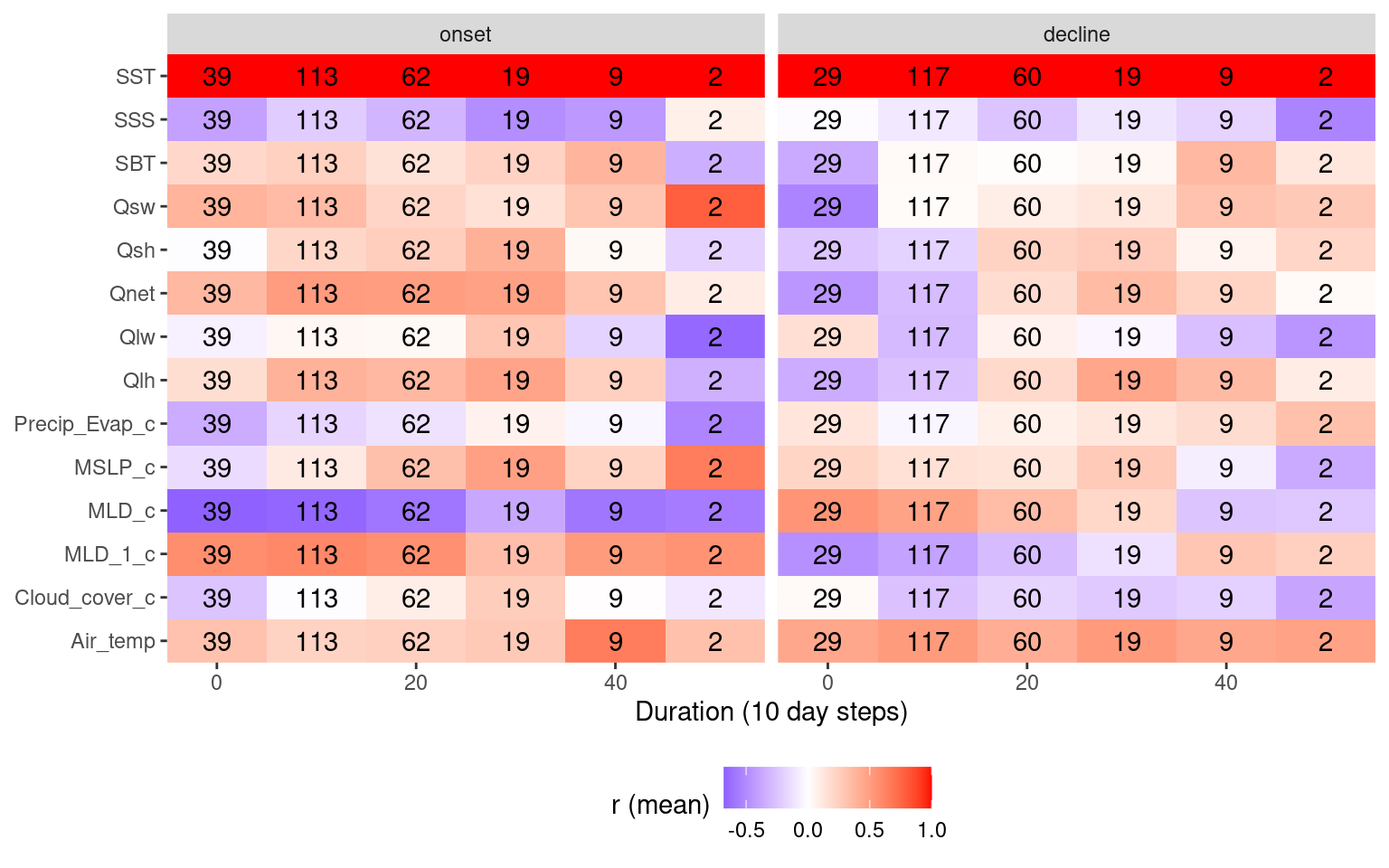
# Heatmap showing average correlations by MHW max intensity
events_cor_prep %>%
  mutate(intensity_max = plyr::round_any(intensity_max, 0.5)) %>%
  group_by(ts, intensity_max) %>%
  mutate(count = n()) %>%
  summarise_if(is.numeric, mean) %>%
  pivot_longer(cols = Air_temp:Qsw) %>%
  filter(name != "sst",
         ts != "full") %>%
  ggplot(aes(x = intensity_max, y = name)) +
  geom_tile(aes(fill = value)) +
  geom_text(aes(label = count)) +
  facet_wrap(~ts) +
  scale_fill_gradient2(low = "blue", high = "red") +
  coord_cartesian(expand = F) +
  labs(y = NULL, x = "Max Intensity (°C; 0.5° steps)", fill = "r (mean)") +
  theme(legend.position = "bottom")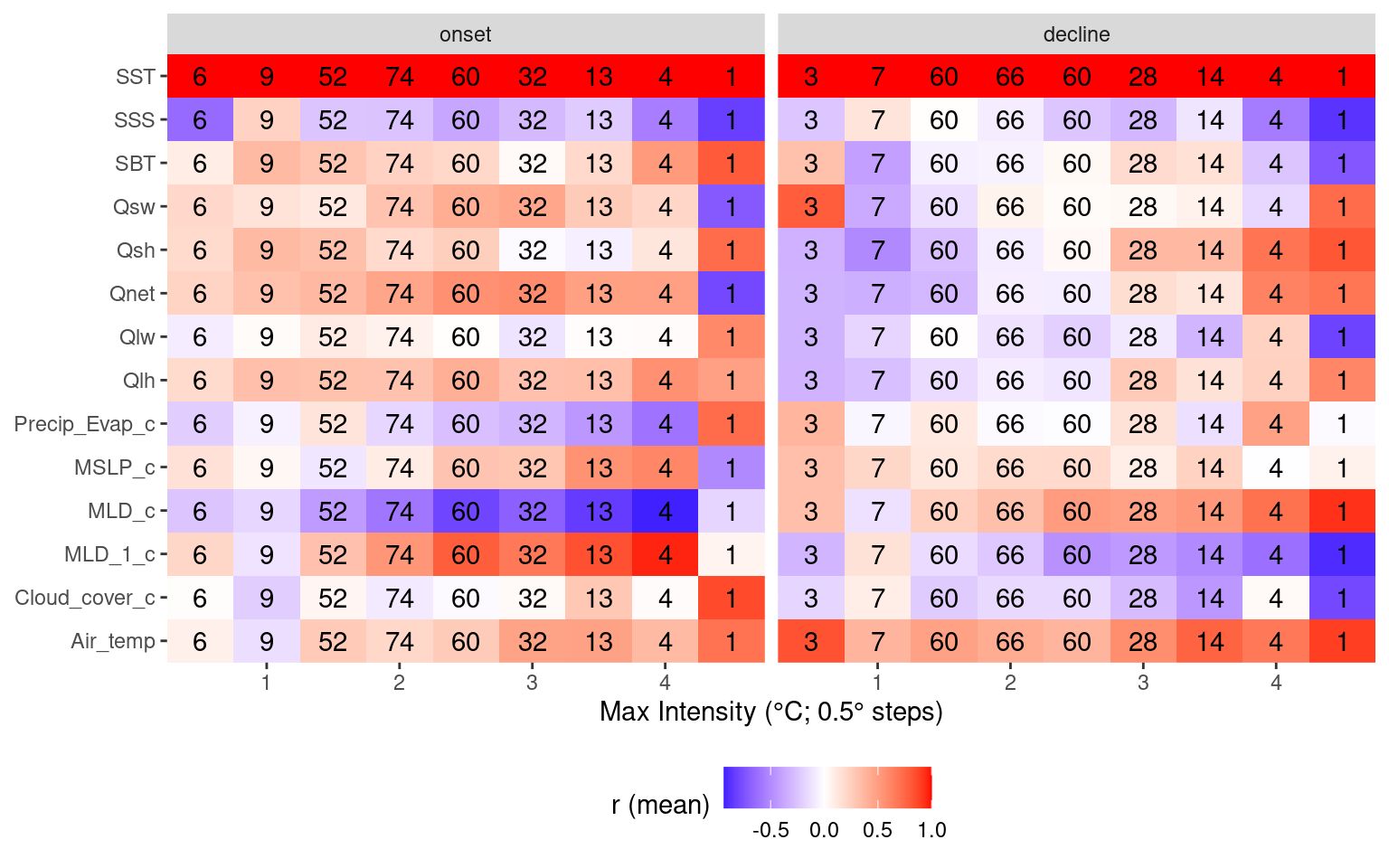
# Heatmap showing average correlations by MHW rate onset
events_cor_prep %>%
  mutate(rate_onset = round(rate_onset, 1)) %>%
  group_by(ts, rate_onset) %>%
  mutate(count = n()) %>%
  summarise_if(is.numeric, mean) %>%
  pivot_longer(cols = Air_temp:Qsw) %>%
  filter(name != "sst",
         ts != "full",
         rate_onset <= 0.75) %>% # Only two is faster than this
  ggplot(aes(x = rate_onset, y = name)) +
  geom_tile(aes(fill = value)) +
  geom_text(aes(label = count)) +
  facet_wrap(~ts) +
  scale_fill_gradient2(low = "blue", high = "red") +
  coord_cartesian(expand = F) +
  labs(y = NULL, x = "Rate of onset (°C; 0.1° steps)", fill = "r (mean)") +
  theme(legend.position = "bottom")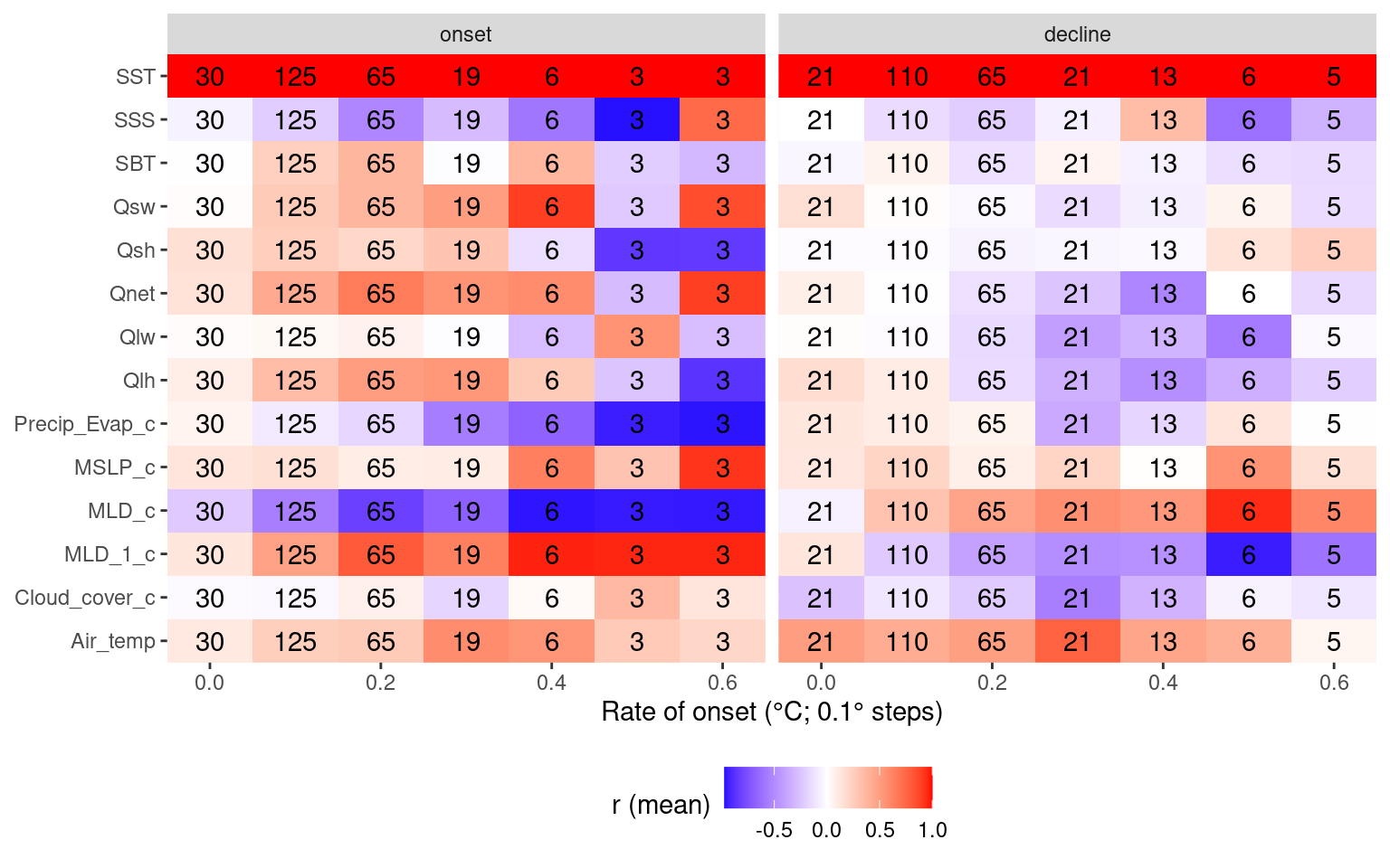
# Heatmap showing average correlations by MHW rate decline
events_cor_prep %>%
  mutate(rate_decline = round(rate_decline, 1)) %>%
  filter(rate_decline <= 0.6) %>% # nip off a couple of outliers
  group_by(ts, rate_decline) %>%
  mutate(count = n()) %>%
  summarise_if(is.numeric, mean) %>%
  pivot_longer(cols = Air_temp:Qsw) %>%
  filter(name != "sst",
         ts != "full") %>%
  ggplot(aes(x = rate_decline, y = name)) +
  geom_tile(aes(fill = value)) +
  geom_text(aes(label = count)) +
  facet_wrap(~ts) +
  scale_fill_gradient2(low = "blue", high = "red") +
  coord_cartesian(expand = F) +
  labs(y = NULL, x = "Rate of decline (°C; 0.1° steps)", fill = "r (mean)") +
  theme(legend.position = "bottom")
Linearity of events
Another observation I made while going through the results in the shiny app was how the onset and decline of events tend to have a better RMSE when the SSTa trend is more linear. My hypothesis is that this is because there is less advective pressure on the dispersion of the heat anomaly, therefore more of the heatflux is responsible for the temperature anomaly. This is a pretty straight forward statement, but I think it is useful in that one may be able to take linearity of SSTa as a proxy for the proportion of heat flux that is responsible for it. So in the chunk below I use simple linear models to create an R2 value for each onset and decline portion of an event. Then I find how close to 1.0 that R2 value is (meaning more linear SSTa) and I see how RMSE changes as R2 improves. I hypothesised that more linear SSTa onset will provide better (lower) RMSE values. The same is likely true for decline but I’m not certain.
# R2 for RMSE vs R2
ALL_cor_R2 <- readRDS("data/ALL_cor.Rda") %>%
  ungroup() %>%
  filter(Parameter1 == "sst", rmse > 0) %>%
  nest_by(region, season, ts) %>%
  summarise(broom::glance(lm(rmse ~ sst_R2, data = data)))

# Scatterplots
readRDS("data/ALL_cor.Rda") %>%
  ungroup() %>%
  filter(Parameter1 == "sst", rmse > 0) %>%
  ggplot(aes(x = sst_R2, y = rmse)) +
  geom_point() +
  geom_smooth(method = "lm") +
  facet_grid(region ~ Parameter2)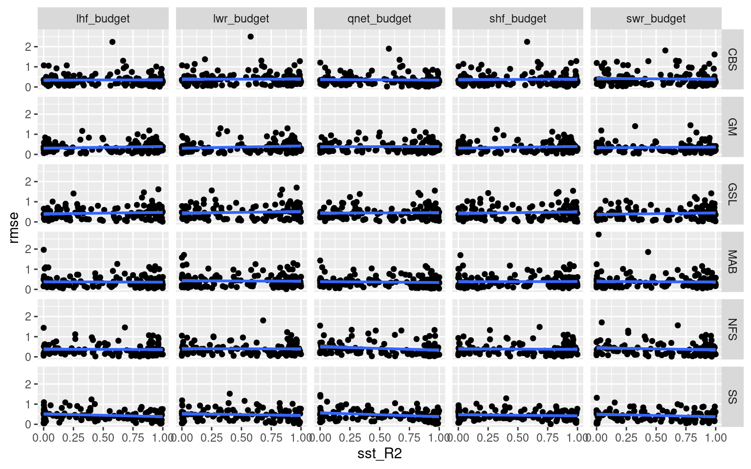
# Boxplots
readRDS("data/ALL_cor.Rda") %>%
  ungroup() %>%
  filter(Parameter1 == "sst", rmse > 0) %>%
  mutate(sst_R2_cut = cut(sst_R2, breaks = c(0, 0.25, 0.5, 0.75,1.0))) %>%
  na.omit() %>%
  ggplot(aes(x = sst_R2_cut, y = rmse)) +
  geom_boxplot() +
  facet_grid(region ~ Parameter2)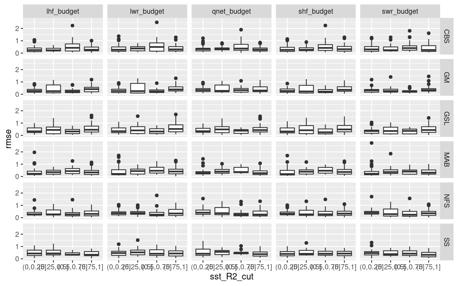
Nope. If there is any relationship it is incredibly noisy. I’ll not be pursuing this further for this project, but I’m not entirely dissuaded from pursuing this avenue of research in the future with a deeper learning approach.
Choice events
There are a lot of results to wade through and though it is clear there are important signals in the results, but it is proving difficult to distill them. One thought is that we don’t need to look at all of the events, just the longest/most intense events with strong r values. This is first done by cutting out all Category I events. We then find strong correlations with long events. There should just be a few.
Once this has been done we group events by their strongest Qx relationship, then find their strongest relationship with the next level of variables (e.g. MLD, MSLP, and so on). Ideally one may find the top four flavours.
# Filter out smol events
events_cor_cat <- events_cor_prep %>%
  left_join(OISST_MHW_cats[,c("region", "event_no", "category")], by = c("region", "event_no")) %>%
  filter(category != "I Moderate", duration >= 21)

# Events with high Qlw correlations at onset
events_cor_cat %>%
  filter(ts == "onset", Qlw >= 0.7)
# A tibble: 3 x 26
# Groups: region [3]
region season event_no duration intensity_mean intensity_max intensity_cumul…
<chr> <fct> <int> <dbl> <dbl> <dbl> <dbl>
1 CBS Summer 36 24 2.71 3.88 65.1
2 GSL Winter 21 69 1.52 2.47 105.
3 MAB Autumn 39 28 2.39 3.30 67.0
# … with 19 more variables: rate_onset <dbl>, rate_decline <dbl>, ts <fct>,
# n_Obs <int>, Air_temp <dbl>, SBT <dbl>, SSS <dbl>, SST <dbl>,
# Cloud_cover_c <dbl>, MSLP_c <dbl>, Precip_Evap_c <dbl>, MLD_c <dbl>,
# MLD_1_c <dbl>, Qnet <dbl>, Qlh <dbl>, Qsh <dbl>, Qlw <dbl>, Qsw <dbl>,
# category <chr># Melt the data frame and find the q term with the highest correlation
# Those are then used to separate events into groups
events_q_onset <- events_cor_cat %>%
filter(ts == "onset") %>%
dplyr::select(region:event_no, ts, Qnet:Qsh) %>%
pivot_longer(cols = Qnet:Qsh, names_to = "var", values_to = "val") %>%
group_by(region, season, event_no) %>%
filter(abs(val) == max(abs(val)))
# With this guide one may then parse out the q groups
events_lhf_p_onset <- events_q_onset %>%
filter(val >= 0, var == "Qlh") %>%
left_join(events_cor_cat) %>%
ungroup() %>%
# unite(region, season, event_no, sep = "_")
mutate(event_no = as.factor(event_no)) %>%
dplyr::select(region:ts, Air_temp:Qsw) %>%
pivot_longer(Air_temp:Qsw) %>%
ggplot(aes(x = event_no, y = name)) +
geom_tile(aes(fill = value)) +
# facet_wrap(~name, scales = "free") +
scale_fill_gradient2(low = "blue", high = "red") +
coord_cartesian(expand = F) +
labs(y = NULL, fill = "r (mean)") +
theme(legend.position = "bottom")
events_lhf_p_onset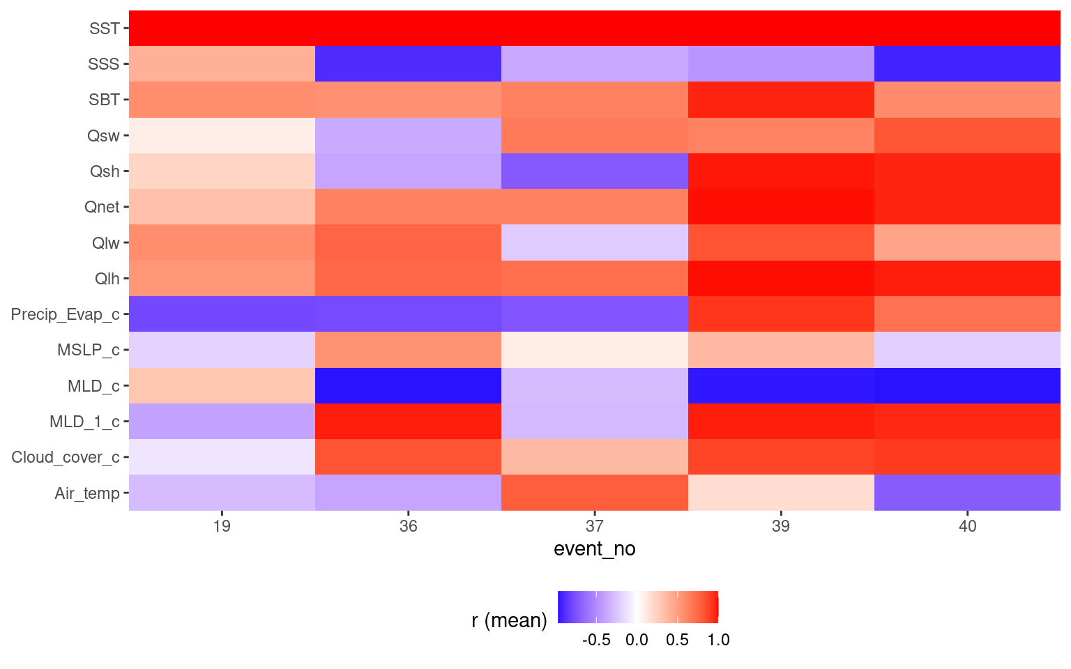
Table
In the following table a more concise summary of the results is presented.
| variable | abbreviation | onset | full | decline | season | region | overall | story |
|---|---|---|---|---|---|---|---|---|
| Air temperature | t2m | Even throughout | Slight positive | Strong positive | Autumn always strong positive for decline. Spring decline has large range. | Stronger positive for GSL and MAB. | Much clearer relationship for decline than onset. | TRUE |
| Total precipitation | tp | Normal with slight positive | Normal distribution | Even throughout | Autumn and Winter slightly more positive with Spring decline usually negative. | Nothing clear. SS and NFS decline most often r ~= 0. | Meh. | FALSE |
| Total evaporation | e | Even throughout | Normal distribution | Strong positive | Spring is the only season that isn’t mostly positive for decline. | SS is the only region not mostly positive for decline. | Important for the decline of events, except often in Spring. | TRUE |
| Precipitation minus evaporation | p_e | Normal with minor positive | Normal with minor positive | Normal with minor positive | Autumn then Winter tend more positive. | MAB decline more positive than others. GM GSL and MAB onset tend more positive. | This value is all over the board. It likely only coincides with MHWs due to something else. | FALSE |
| Prec – evap (cumulative) | p_e_cum | Strong negative and positive | Normal | Flat with positive tail | Spring then Summer strong negative onset. Autumn strong positive onset and decline. | GSL tends negative for decline while others tend positive. Very large ranges overall. | There is an important signal in the differences between Spring-Summer and Autumn. | TRUE |
| Air Northerly | v10 | Three hump | Normal distribution | Three hump | Large spread for all seasons with Autumn tending towards positive for onset and decline. | Not much difference. NFS tends a bit more towards positive onset and decline than others. | There are some signals in there, but they are not clear. | FALSE |
| Air Easterly | u10 | Slight positive | Normal distribution | Slight negative | Least amount of range in Autumn onset. | GM tends to have the least range and be the most negative for onset and decline. | Slight positive onset and slight negative decline imply this vaguely shows a thermal gradient. | FALSE |
| Wind speed | wind_spd | Normal but flat | Normal | Negative | Autumn onset tends positive while everything else tends negative. Summer decline more negative. | GM and MAB tend more negative for decline. | A smol signal for the GM and MAB showing decline negative with wind speed. | FALSE |
| Total cloud cover | tcc | Normal but positive | Normal but positive | Normal but positive | Spring onset tends most positive. | GM and NFS full tend more positive. MAB decline tends more positive. | Meh. | FALSE |
| Total cloud cover (cumulative) | tcc_cum | Strong positive with negative tail | Normal | Negative and positive | Autumn onset tends much more positive. Spring decline tends more negative. | Large ranges in onset. GSL tends much more negative for decline. | May be important for GSL events due to SWR importance there. | FALSE |
| Mean sea level pressure | msl | Strong negative with positive tail | Slight negative to normal | Even with positive tail | Autumn is much more negative for onset and decline. Spring and Summer onset tend positive. | GM and NFS more positive for decline. | Decrease in MSLP is often important for the onset of events | TRUE |
| Mean sea level pressure (cumulative) | msl_cum | Strong negative and positive | Normal but flat | Strong positive with small negative tail | Full range in onset and decline for all seasons except positive Spring onset. Autumn onset tends negative. | Full range for all. GM decline tends positive. CBS onset tends negative, NFS and SS onset tend positive. | Stronger signals than for MSLP non-cumulative. | TRUE |
| Sea surface height | ssh | Even throughout | Slight negative | Positive tail | Autumn onset and decline tend negative. | GM decline positive. | The strong positive signal for decline implies a height anomaly (i.e. an eddy) leaving the area. | TRUE |
| Current Northerly | v | Normal but flat | Normal distribution | Positive with small negative tail | Not much difference. Winter onset tends more negative. | GM onset and decline tend more positive. | Meh. | FALSE |
| Current Easterly | u | Normal with positive tail | Normal distribution | Slight three hump | Autumn decline tends positive while Summer tends negative. | NFS onset tends most positive. | Possibly something there for onset of events in NFS. | FALSE |
| Current speed | cur_spd | Flat but slight negative | Normal but negative | Flat but negative | Autumn onset tends to be positive while everything else tends negative. | GSL decline tends much more negative while MAB decline tends positive. | The positive decline for MAB implies the importance of advection for events. | FALSE |
| Sea surface salinity | sss | Strong negative with positive tail | Negative | Strong negative with positive tail | Summer then Autumn tend more negative. Largest range on Winter. | GSL much more negative for onset+full+decline. CBS onset strong negative. GM decline strong negative. | Strong negative mixed in with noise. Large differences between regions. | TRUE |
| Mixed layer depth | mld | Strong negative with positive tail | Negative | Strong negative with minor positive tail | Strong negative decline for all but Summer. Summer onset negative with large Spring and Winter range. | Strong negative for all but CBA and SS with large range. All negative onset but large ranges. | The decline of a MHW in Summer or the onset in Winter + Spring doesn’t seem as tied to MLD. | TRUE |
| Bottom temperature | bottomT | Strong positive with minor negative tail | Normal but flat | Strong positive with small negative tail | Large ranges with strong positive Autumn onset. | Strong positive onset for MAB + GM. CBS decline tends negative. | MHWs in Autumn generally have high bottom temps at onset | TRUE |
| Latent heat flux | mslhf_mld | Strong positive | Positive | Strong positive | Very strong positive onset+full+decline for Autumn. Large range in onset+decline in Spring. | Strong positive onset for MAB. | This variable is almost always important for onset and decline, especially in Autumn. | TRUE |
| Sensible heat flux | msshf_mld | Strong positive with negative tail | Flat | Strong positive with minor negative tail | Strong positive onset for Autumn + Winter and negative for Spring + Summer. | Some difference in tendency but similar ranges for all regions. | Very large differences in negative or positive correlations based on seasons. | TRUE |
| Longwave radiation | msnlwrf_mld | Strong positive with minor negative tail | Slight positive | Flat with positive tail | Positive onset tendency with Autumn much stronger. Spring + Summer decline tend negative. | Strong positive onset for MAB + GM. | Autumn may be significantly different from Spring. | TRUE |
| Shortwave radiation | msnswrf_mld | Negative with strong positive tail | Slight negative | Positive and negative | Strong negative onset for Autumn. Large range for everything else. | Strong negative onset for GM but largest spread for MAB. | A decrease in SWR in Autumn leads to MHWs, implying cloud cover or some other LHF mechanism. | TRUE |
| Net heat flux | qnet_mld | Very strong positive | Positive | Strong positive with minor negative tail | Autumn has strongest positive onset+full+decline. Spring decline has large range with negative tendency. | MAB strong positive onset + decline. All others tend positive with larger range in decline for GM. | All regions and seasons tend strong positive but with some notable outliers. | TRUE |
References
Chen, K., Kwon, Y.-O., and Gawarkiewicz, G. (2016). Interannual variability of winter-spring temperature in the middle atlantic bight: Relative contributions of atmospheric and oceanic processes. Journal of Geophysical Research: Oceans 121, 4209–4227.
sessionInfo()R version 4.0.3 (2020-10-10)
Platform: x86_64-pc-linux-gnu (64-bit)
Running under: Ubuntu 20.04.1 LTS
Matrix products: default
BLAS: /usr/lib/x86_64-linux-gnu/openblas-pthread/libblas.so.3
LAPACK: /usr/lib/x86_64-linux-gnu/openblas-pthread/liblapack.so.3
locale:
[1] LC_CTYPE=en_CA.UTF-8 LC_NUMERIC=C
[3] LC_TIME=en_CA.UTF-8 LC_COLLATE=en_CA.UTF-8
[5] LC_MONETARY=en_CA.UTF-8 LC_MESSAGES=en_CA.UTF-8
[7] LC_PAPER=en_CA.UTF-8 LC_NAME=C
[9] LC_ADDRESS=C LC_TELEPHONE=C
[11] LC_MEASUREMENT=en_CA.UTF-8 LC_IDENTIFICATION=C
attached base packages:
[1] parallel stats graphics grDevices utils datasets methods
[8] base
other attached packages:
[1] doParallel_1.0.16 iterators_1.0.13 foreach_1.5.1 FNN_1.1.3
[5] Metrics_0.1.4 yasomi_0.3 proxy_0.4-24 e1071_1.7-4
[9] ggraph_2.0.4 correlation_0.5.0 tidync_0.2.4 heatwaveR_0.4.5
[13] lubridate_1.7.9.2 data.table_1.13.6 forcats_0.5.0 stringr_1.4.0
[17] dplyr_1.0.2 purrr_0.3.4 readr_1.4.0 tidyr_1.1.2
[21] tibble_3.0.4 ggplot2_3.3.3 tidyverse_1.3.0
loaded via a namespace (and not attached):
[1] colorspace_2.0-0 ggsignif_0.6.0 ellipsis_0.3.1 class_7.3-17
[5] rio_0.5.16 rprojroot_2.0.2 parameters_0.10.1 fs_1.5.0
[9] rstudioapi_0.13 ggpubr_0.4.0 farver_2.0.3 graphlayouts_0.7.1
[13] ggrepel_0.9.0 fansi_0.4.1 xml2_1.3.2 splines_4.0.3
[17] codetools_0.2-18 ncdf4_1.17 knitr_1.30 polyclip_1.10-0
[21] jsonlite_1.7.2 workflowr_1.6.2 broom_0.7.3 dbplyr_2.0.0
[25] ggforce_0.3.2 effectsize_0.4.1 compiler_4.0.3 httr_1.4.2
[29] backports_1.2.1 Matrix_1.2-18 assertthat_0.2.1 cli_2.2.0
[33] later_1.1.0.1 tweenr_1.0.1 htmltools_0.5.1 tools_4.0.3
[37] igraph_1.2.6 gtable_0.3.0 glue_1.4.2 Rcpp_1.0.5
[41] carData_3.0-4 cellranger_1.1.0 RNetCDF_2.4-2 vctrs_0.3.6
[45] nlme_3.1-150 insight_0.12.0 xfun_0.20 openxlsx_4.2.3
[49] rvest_0.3.6 lifecycle_0.2.0 ncmeta_0.3.0 rstatix_0.6.0
[53] MASS_7.3-53 scales_1.1.1 tidygraph_1.2.0 hms_1.0.0
[57] promises_1.1.1 yaml_2.2.1 curl_4.3 gridExtra_2.3
[61] stringi_1.5.3 highr_0.8 bayestestR_0.8.0 zip_2.1.1
[65] rlang_0.4.10 pkgconfig_2.0.3 lattice_0.20-41 evaluate_0.14
[69] labeling_0.4.2 cowplot_1.1.1 tidyselect_1.1.0 plyr_1.8.6
[73] magrittr_2.0.1 R6_2.5.0 generics_0.1.0 DBI_1.1.1
[77] mgcv_1.8-33 pillar_1.4.7 haven_2.3.1 whisker_0.4
[81] foreign_0.8-79 withr_2.3.0 abind_1.4-5 modelr_0.1.8
[85] crayon_1.3.4 car_3.0-10 utf8_1.1.4 rmarkdown_2.6
[89] viridis_0.5.1 grid_4.0.3 readxl_1.3.1 git2r_0.28.0
[93] reprex_0.3.0 digest_0.6.27 httpuv_1.5.5 munsell_0.5.0
[97] viridisLite_0.3.0